Explainers

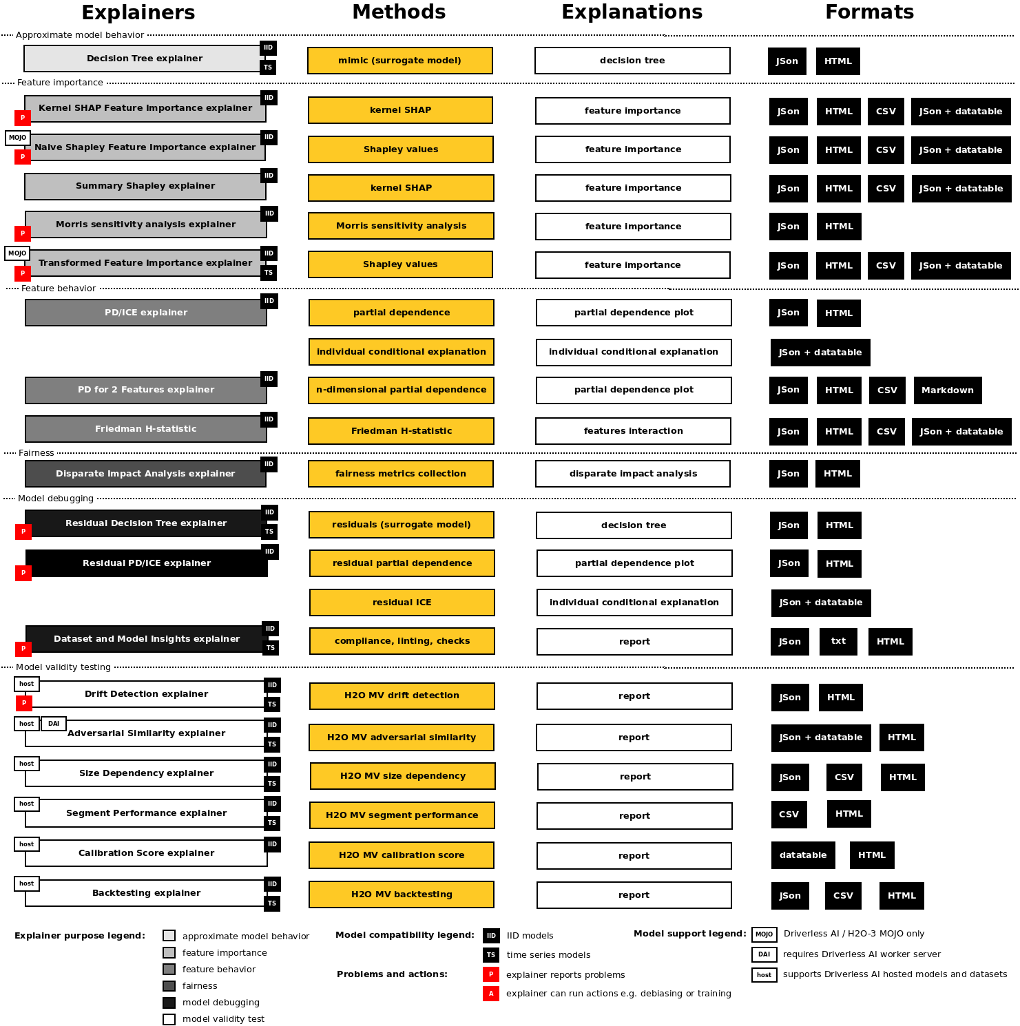
H2O Eval Studio explainers:

• Approximate model behavior

  • Surrogate Decision Tree Explainer

• Feature importance

  • Shapley Summary Plot for Original Features (Naive Shapley Method) Explainer

  • Shapley Values for Original Features (Kernel SHAP Method) Explainer

  • Shapley Values for Original Features of MOJO Models (Naive Method) Explainer

  • Shapley Values for Transformed Features of MOJO Models Explainer

  • Morris sensitivity analysis Explainer

• Feature behavior

  • Partial Dependence/Individual Conditional Expectations (PD/ICE) Explainer

  • Partial Dependence for 2 Features Explainer

  • Friedman’s H-statistic Explainer

• Fairness

  • Disparate Impact Analysis (DIA) Explainer

• Model debugging

  • Residual Surrogate Decision Tree Explainer

  • Residual Partial Dependence/Individual Conditional Expectations (PD/ICE) Explainer

  • Dataset and Model Insights Explainer

• Model validity testing

  • Adversarial Similarity Explainer

  • Backtesting Explainer

  • Calibration Score explainer

  • Drift Detection Explainer

  • Segment Performance Explainer

  • Size Dependency Explainer

Name	D/M	IID	TS	R	B	M	G	L	p()	r()	DAI	autoML
Decision Tree	M	✓	✓	✓	✓	✓	✓	✓	✓	❌	❌	❌
Kernels SHAP Feature Importance	M	✓	✓	✓	✓	✓	✓	✓	✓	❌	❌	❌
Naive Shapley Feature Importance	M	✓	✓	✓	✓	✓	✓	✓	✓	❌	❌	❌
Summary Shapley	M	✓	✓	✓	✓	✓	✓	❌	✓	❌	❌	❌
Morris Sensitivity Analysis	M	✓	✓	✓	✓	❌	✓	❌	✓	❌	❌	❌
Transformed Feature Importance	M	✓	✓	✓	✓	✓	✓	✓	✓	❌	❌	❌
PD/ICE	M	✓	✓	✓	✓	✓	✓	✓	✓	❌	❌	❌
PD/ICE for 2 Features	M	✓	✓	✓	✓	❌	✓	❌	✓	❌	❌	❌
Friedman H-statistic	M	✓	✓	✓	✓	❌	✓	❌	✓	❌	❌	❌
Disparate Impact Analysis	M	✓	✓	✓	✓	❌	✓	❌	✓	❌	❌	❌
Residual Decision Tree	M	✓	✓	✓	✓	✓	✓	✓	✓	❌	❌	❌
Residual PD/ICE	M	✓	✓	✓	✓	✓	✓	✓	✓	❌	❌	❌
Dataset and Model Insights	D+M	✓	✓	✓	✓	✓	✓	❌	✓	❌	❌	❌
Adversarial Similarity	D+rD	✓	✓	✓	✓	✓	✓	❌	❌	❌	✓	✓
Backtesting	rM	✓	✓	✓	✓	✓	✓	❌	✓	✓	✓	❌
Calibration Score	rM	✓	✓	❌	✓	✓	✓	❌	✓	❌	✓	❌
Drift Detection	D+rD	✓	✓	✓	✓	✓	✓	❌	❌	❌	✓	❌
Segment Performance	rM	✓	✓	✓	✓	✓	✓	❌	✓	❌	✓	❌
Size Dependency	rM	✓	✓	✓	✓	✓	✓	❌	✓	❌	✓	❌

Legend:

• D/M

  • Explainer can explain local dataset (D), remote dataset hosted by Driverless AI (rD), local model (M) or remote model hosted by Driverless AI (rM).

• IID

  • Explainer can explain IID models (with independent and identically distributed variables).

• TS

  • Explainer can explain time series models.

• R

  • Explainer can explain models for regression problems.

• B

  • Explainer can explain models for binomial classification problems.

• M

  • Explainer can explain models for multinomial classification problems.

• Global

  • Explainer provides global explanations.

• Local

  • Explainer provides local explanations.

• p()

  • Model must support predict() method.

• r()

  • Model must support retrain() or refit() method.

• DAI

  • Explainer requires Driverless AI connection of the server which may host explained datasets and/or models.

• autoML

  • Explainer requires connection to autoML Driverless AI worker in order to run experiments.

Explainer Parameters

Explainers can be parameterized using the parameters documented in the sections below. These parameters are explainer specific and can be passed to explainers using the Python API as follows:

interpretation = interpret.run_interpretation(
    dataset=dataset_path,
    model=mock_model,
    target_col=target_col,
    explainers=[
        commons.ExplainerToRun(
            explainer_id=explainer.PdIceExplainer.explainer_id(),
            params={
                explainer.PdIceExplainer.PARAM_MAX_FEATURES: param_max_features,
                explainer.PdIceExplainer.PARAM_GRID_RESOLUTION: param_bins,
            },
        )
    ],
    ...
)

In the example above, max_features and grid_parameters parameters are passed to the PdIceExplainer. An instance of the ExplainerToRun class is used to specify explainer ID and its parameters, which are passed in a dictionary, where the key is string identifier of the parameter and value is the parameter value.

Similarly parameters can be passed to the explainers using the command line (CLI) interface:

h2o-sonar run interpretation
  --dataset=dataset.csv
  --model=model.pickle
  --target-col=PROFIT
  --explainers=h2o_sonar.explainers.pd_ice_explainer.PdIceExplainer
  --explainers-pars=
    "{'h2o_sonar.explainers.pd_ice_explainer.PdIceExplainer':{'max_features': 5}}"

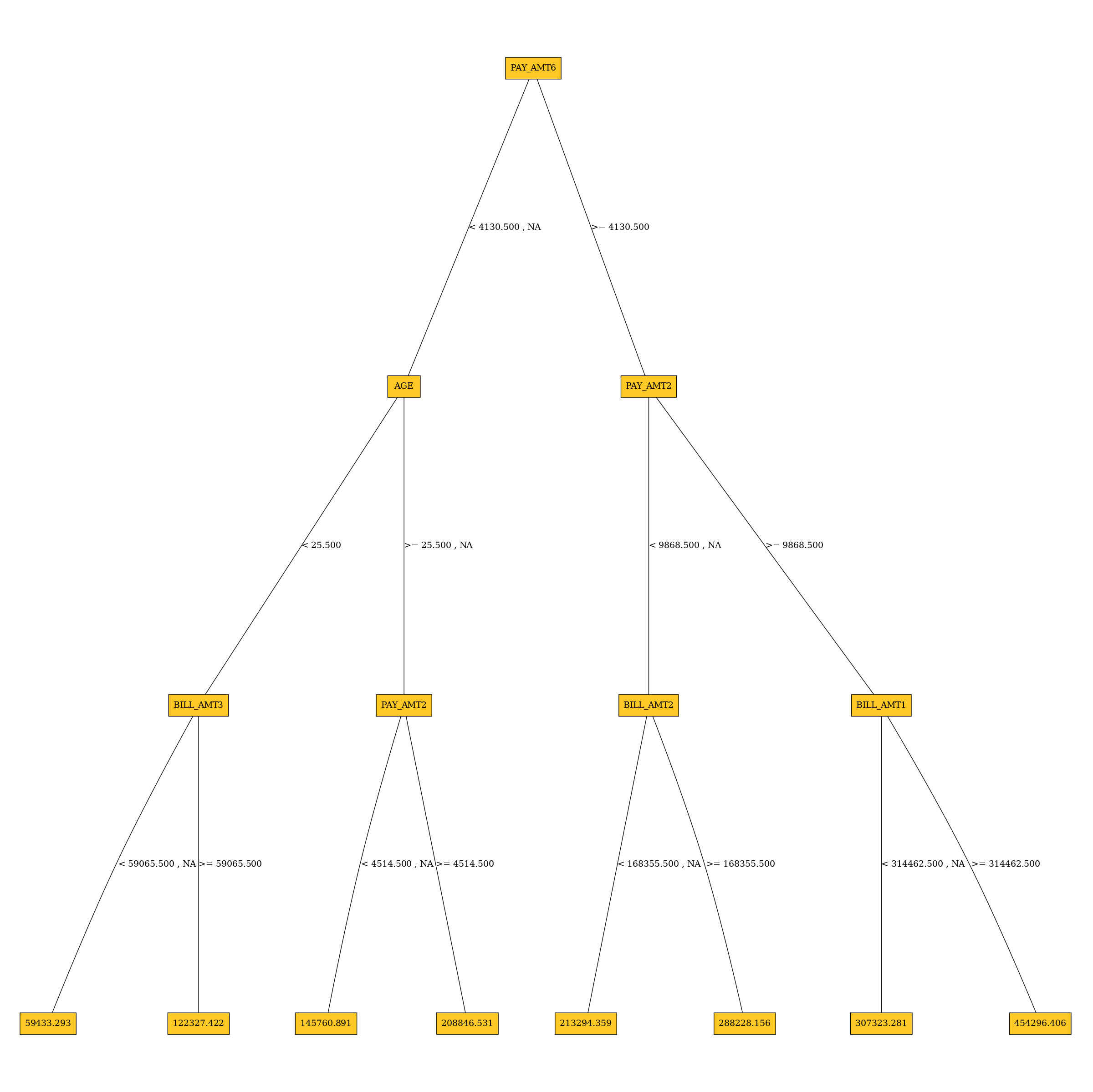
Surrogate Decision Tree Explainer

The decision tree surrogate is an approximate overall flow chart of the model, created by training a simple decision tree on the original inputs and the predictions of the model.

Explainer parameters:

• debug_residuals

  • Debug model residuals.

• debug_residuals_class

  • Class for debugging classification model logloss residuals, empty string for debugging regression model residuals.

• dt_tree_depth

  • Decision tree depth.

• nfolds

  • Number of CV folds.

• qbin_cols

  • Quantile binning columns.

• qbin_count

  • Quantile bins count.

• categorical_encoding

  • Categorical encoding - specify one of the following encoding schemes for handling of categorical features:

    • AUTO: 1 column per categorical feature.

    • Enum Limited: Automatically reduce categorical levels to the most prevalent ones during training and only keep the top 10 most frequent levels.

    • One Hot Encoding: N+1 new columns for categorical features with N levels.

    • Label Encoder: Convert every enum into the integer of its index (for example, level 0 -> 0, level 1 -> 1, etc.).

    • Sort by Response: Reorders the levels by the mean response (for example, the level with lowest response -> 0, the level with second-lowest response -> 1, etc.).

Explainer result directory description:

explainer_h2o_sonar_explainers_dt_surrogate_explainer_DecisionTreeSurrogateExplainer_89c7869d-666d-4ba2-ba84-cf1aa1b903bd
├── global_custom_archive
│   ├── application_zip
│   │   └── explanation.zip
│   └── application_zip.meta
├── global_decision_tree
│   ├── application_json
│   │   ├── dt_class_0.json
│   │   └── explanation.json
│   └── application_json.meta
├── local_decision_tree
│   ├── application_json
│   │   └── explanation.json
│   └── application_json.meta
├── log
│   └── explainer_run_89c7869d-666d-4ba2-ba84-cf1aa1b903bd.log
├── result_descriptor.json
└── work
    ├── dtModel.json
    ├── dtpaths_frame.bin
    ├── dtPathsFrame.csv
    ├── dtsurr_mojo.zip
    ├── dtSurrogate.json
    └── dt_surrogate_rules.zip

• explainer_.../work/dtSurrogate.json

  • Decision tree in JSon format.

• explainer_.../work/dt_surrogate_rules.zip

  • Decision tree rules (in Python and text format) stored in ZIP archive.

• explainer_.../work/dtpaths_frame.bin

  • Decision tree paths stored as datatable frame.

• explainer_.../work/dtPathsFrame.csv

  • Decision tree paths stored as CSV file.

• explainer_.../work/dtsurr_mojo.zip

  • Decision tree model stored as zipped H2O-3 MOJO.

• explainer_.../work/dtModel.json

  • Decision tree model in JSon format.

Explanations created by the explainer:

• global_custom_archive

  • ZIP archive with explainer artifacts.

• global_decision_tree

  • Decision tree explanation in the JSon format.

• local_decision_tree

  • Local (per dataset row) decision tree explanations in the JSon format.

See also:

• Decision Tree Surrogate Explainer Demo

• Interpretation Directory Structure

• Explainer Parameters

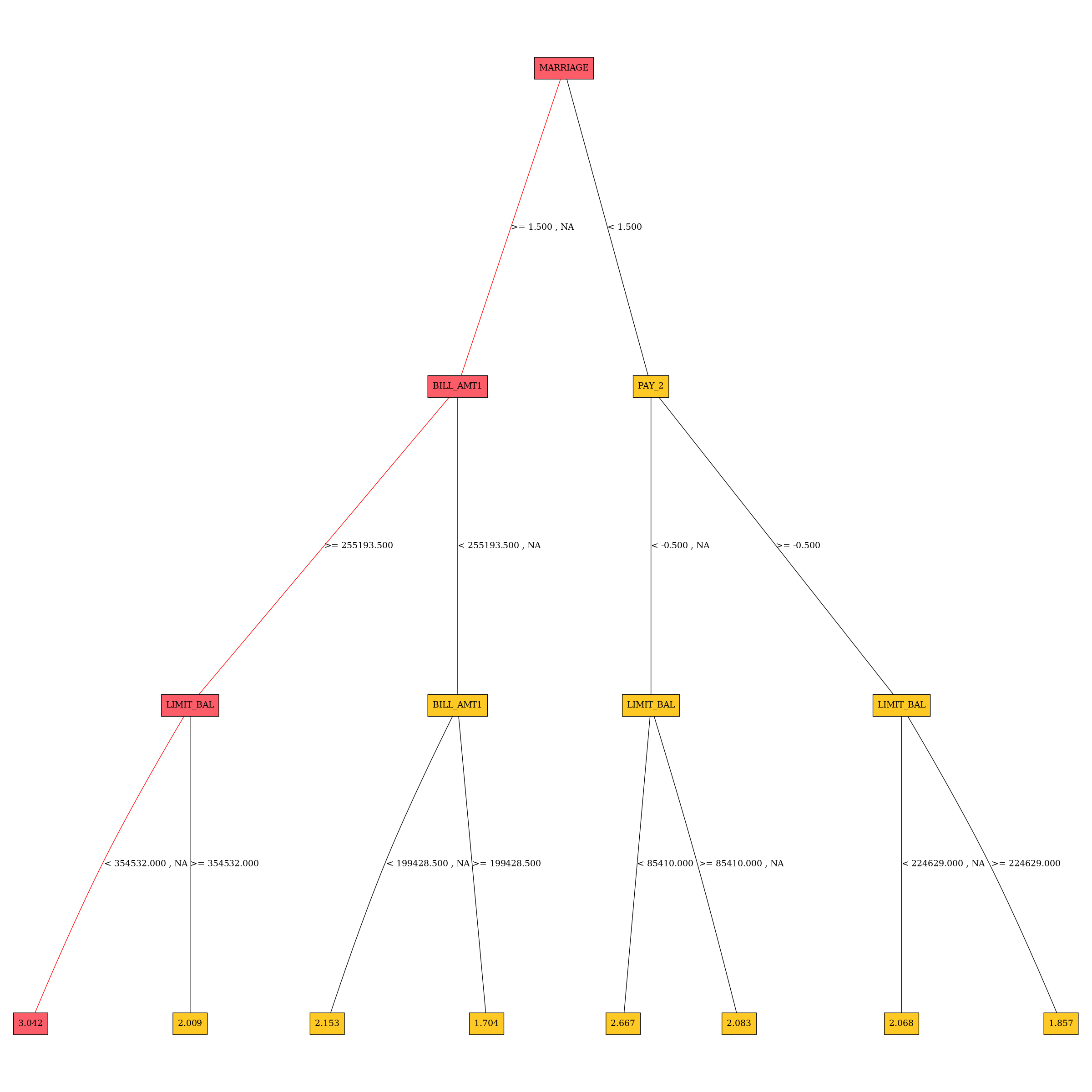
Residual Surrogate Decision Tree Explainer

The residual surrogate decision tree predicts which paths in the tree (paths explain approximate model behavior) lead to highest or lowest error. The residual surrogate decision tree is created by training a simple decision tree on the residuals of the predictions of the model. Residuals are differences between observed and predicted values which can be used as targets in surrogate models for the purpose of model debugging. The method used to calculate residuals varies depending on the type of problem. For classification problems, logloss residuals are calculated for a specified class. For regression problems, residuals are determined by calculating the square of the difference between targeted and predicted values.”

Explainer parameters:

• debug_residuals_class

  • Class for debugging classification model logloss residuals, empty string for debugging regression model residuals.

• dt_tree_depth

  • Decision tree depth.

• nfolds

  • Number of CV folds.

• qbin_cols

  • Quantile binning columns.

• qbin_count

  • Quantile bins count.

• categorical_encoding

  • Categorical encoding - specify one of the following encoding schemes for handling of categorical features:

    • AUTO: 1 column per categorical feature.

    • Enum Limited: Automatically reduce categorical levels to the most prevalent ones during training and only keep the top 10 most frequent levels.

    • One Hot Encoding: N+1 new columns for categorical features with N levels.

    • Label Encoder: Convert every enum into the integer of its index (for example, level 0 -> 0, level 1 -> 1, etc.).

    • Sort by Response: Reorders the levels by the mean response (for example, the level with lowest response -> 0, the level with second-lowest response -> 1, etc.).

Explainer result directory description:

explainer_h2o_sonar_explainers_residual_dt_surrogate_explainer_ResidualDecisionTreeSurrogateExplainer_606aa553-e0f4-4a6f-a6b6-366955ca938d
├── global_custom_archive
│   ├── application_zip
│   │   └── explanation.zip
│   └── application_zip.meta
├── global_decision_tree
│   ├── application_json
│   │   ├── dt_class_0.json
│   │   └── explanation.json
│   └── application_json.meta
├── global_html_fragment
│   ├── text_html
│   │   ├── dt-class-0.png
│   │   └── explanation.html
│   └── text_html.meta
├── local_decision_tree
│   ├── application_json
│   │   └── explanation.json
│   └── application_json.meta
├── log
│   └── explainer_run_606aa553-e0f4-4a6f-a6b6-366955ca938d.log
├── result_descriptor.json
└── work
    ├── dt-class-0.dot
    ├── dt-class-0.dot.pdf
    ├── dtModel.json
    ├── dtpaths_frame.bin
    ├── dtPathsFrame.csv
    ├── dtsurr_mojo.zip
    ├── dtSurrogate.json
    └── dt_surrogate_rules.zip

• explainer_.../work/dtSurrogate.json

  • Decision tree in JSon format.

• explainer_.../work/dt_surrogate_rules.zip

  • Decision tree rules (in Python and text format) stored in ZIP archive.

• explainer_.../work/dtpaths_frame.bin

  • Decision tree paths stored as datatable frame.

• explainer_.../work/dtPathsFrame.csv

  • Decision tree paths stored as CSV file.

• explainer_.../work/dtsurr_mojo.zip

  • Decision tree model stored as zipped H2O-3 MOJO.

• explainer_.../work/dtModel.json

  • Decision tree model in JSon format.

Explanations created by the explainer:

• global_custom_archive

  • ZIP archive with explainer artifacts.

• global_decision_tree

  • Decision tree explanation in the JSon format.

• local_decision_tree

  • Local (per dataset row) decision tree explanations in the JSon format.

Problems reported by the explainer:

• Path leading to the highest error

  • The explainer reports residual decision tree path that leads to the highest error. This path should be investigated to determine whether it indicates a problem with the model.

  • Problem severity: LOW.

See also:

• Residual Decision Tree Surrogate Explainer Demo

• Interpretation Directory Structure

• Explainer Parameters

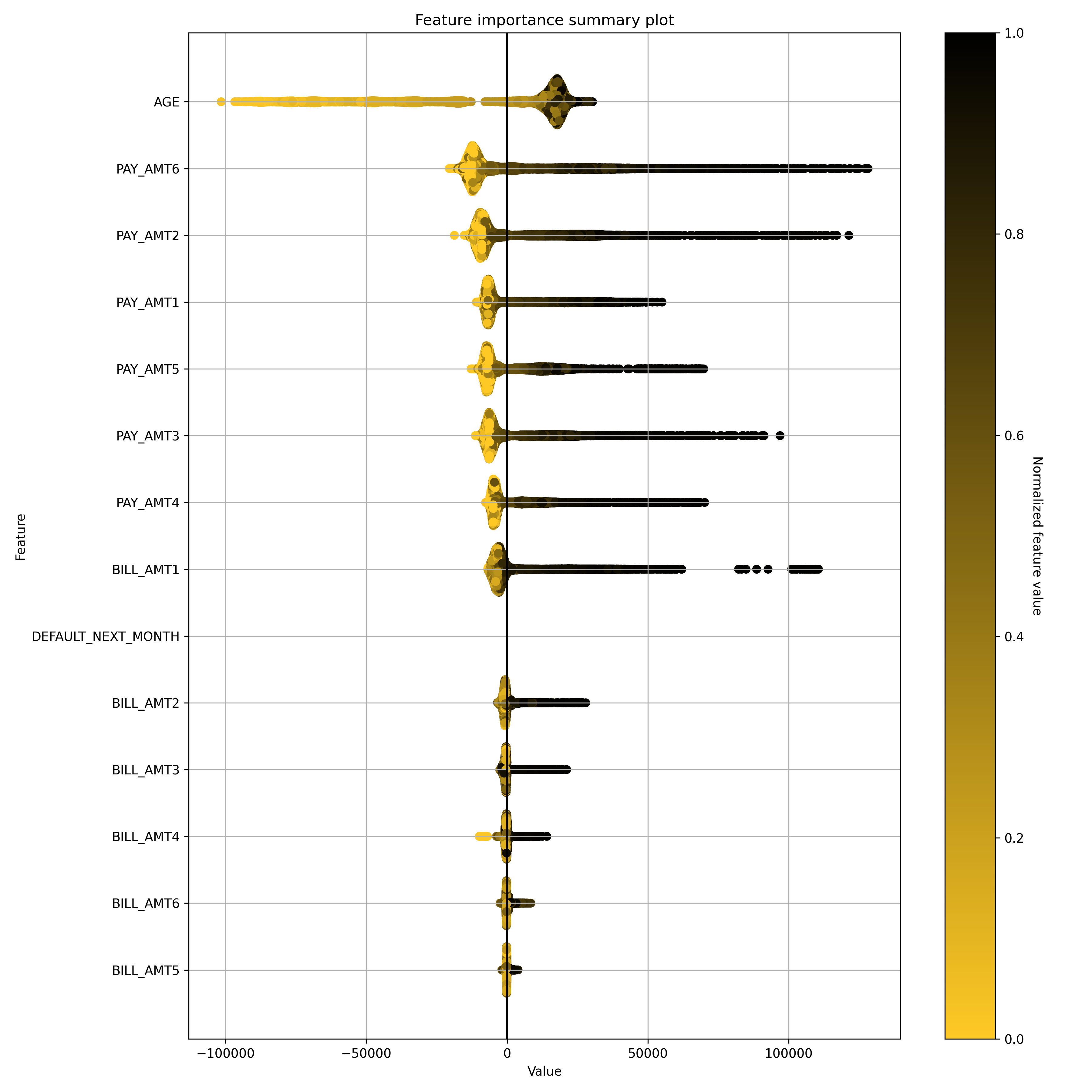
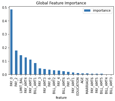
Shapley Summary Plot for Original Features (Naive Shapley Method) Explainer

Shapley explanations are a technique with credible theoretical support that presents consistent global and local feature contributions.

The Shapley Summary Plot shows original features versus their local Shapley values on a sample of the dataset. Feature values are binned by Shapley values and the average normalized feature value for each bin is plotted. The legend corresponds to numeric features and maps to their normalized value - yellow is the lowest value and deep orange is the highest. You can also get scatter plot of the actual numeric feature values versus their corresponding Shapley values. Categorical features are shown in grey and do not provide an actual-value scatter plot.

Notes:

• The Shapley Summary Plot only shows original features that are used in the model.

• The dataset sample size and the number of bins can be updated in the interpretation parameters.

• If feature engineering is turned off and there is no sampling, then the Naive Shapley values should match the transformed Shapley values.

Explainer parameters:

• sample_size

  • Sample size (default is 100 000).

• max_features

  • Maximum number of features to be shown in the plot.

• x_shapley_resolution

  • X-axis resolution (number of Shapley values bins).

• enable_drill_down_charts

  • Enable creation of per-feature Shapley/feature value scatter plots.

Explainer result directory description:

explainer_h2o_sonar_explainers_summary_shap_explainer_SummaryShapleyExplainer_36d41c37-7641-4519-9358-a7ddc947f704
├── global_summary_feature_importance
│   ├── application_json
│   │   ├── explanation.json
│   │   ├── feature_0_class_0.png
│   │   ├── feature_10_class_0.png
│   │   ├── feature_11_class_0.png
│   │   ├── feature_12_class_0.png
│   │   ├── feature_13_class_0.png
│   │   ├── feature_14_class_0.png
│   │   ├── feature_15_class_0.png
│   │   ├── feature_16_class_0.png
│   │   ├── feature_17_class_0.png
│   │   ├── feature_18_class_0.png
│   │   ├── feature_19_class_0.png
│   │   ├── feature_1_class_0.png
│   │   ├── feature_20_class_0.png
│   │   ├── feature_21_class_0.png
│   │   ├── feature_22_class_0.png
│   │   ├── feature_23_class_0.png
│   │   ├── feature_2_class_0.png
│   │   ├── feature_3_class_0.png
│   │   ├── feature_4_class_0.png
│   │   ├── feature_5_class_0.png
│   │   ├── feature_6_class_0.png
│   │   ├── feature_7_class_0.png
│   │   ├── feature_8_class_0.png
│   │   ├── feature_9_class_0.png
│   │   ├── summary_feature_importance_class_0_offset_0.json
│   │   ├── summary_feature_importance_class_0_offset_1.json
│   │   └── summary_feature_importance_class_0_offset_2.json
│   ├── application_json.meta
│   ├── application_vnd_h2oai_json_datatable_jay
│   │   ├── explanation.json
│   │   └── summary_feature_importance_class_0.jay
│   ├── application_vnd_h2oai_json_datatable_jay.meta
│   ├── text_markdown
│   │   ├── explanation.md
│   │   └── shapley-class-0.png
│   └── text_markdown.meta
├── log
│   └── explainer_run_36d41c37-7641-4519-9358-a7ddc947f704.log
├── result_descriptor.json
└── work
    ├── raw_shapley_contribs_class_0.jay
    ├── raw_shapley_contribs_index.json
    ├── report.md
    └── shapley-class-0.png

• explainer_.../work/report.md

  • Markdown report with per-class summary Shapley feature importance charts (shapley-class-<class number>.png).

• explainer_.../work/raw_shapley_contribs_index.json

  • Per model class Shapley contributions JSon index - it references datatable .jay frame with the contributions for each class of the model.

Explanations created by the explainer:

• global_summary_feature_importance

  • Summary original feature importance explanation in Markdown (text and global chart), JSon (includes drill-down scatter plots) and datatable formats.

See also:

• Summary Shapley Explainer Demo

• Interpretation Directory Structure

• Explainer Parameters

Shapley Values for Original Features (Kernel SHAP Method) Explainer

Shapley explanations are a technique with credible theoretical support that presents consistent global and local variable contributions. Local numeric Shapley values are calculated by tracing single rows of data through a trained tree ensemble and aggregating the contribution of each input variable as the row of data moves through the trained ensemble. For regression tasks, Shapley values sum to the prediction of the Driverless AI model. For classification problems, Shapley values sum to the prediction of the Driverless AI model before applying the link function. Global Shapley values are the average of the absolute Shapley values over every row of a dataset. Shapley values for original features are calculated with the Kernel Explainer method, which uses a special weighted linear regression to compute the importance of each feature. More information about Kernel SHAP is available at A Unified Approach to Interpreting Model Predictions.

Explainer parameters:

• sample_size

  • Sample size (default is 100 000).

• sample

  • Whether to sample Kernel SHAP (default is True).

• nsample

  • Number of times to re-evaluate the model when explaining each prediction with Kernel Explainer. Default is determined internally.’auto’ or int. Number of times to re-evaluate the model when explaining each prediction. More samples lead to lower variance estimates of the SHAP values. The ‘auto’ setting uses nsamples = 2 * X.shape[1] + 2048. This setting is disabled by default and runtime determines the right number internally.

• L1

  • L1 regularization for Kernel Explainer. ” ‘num_features(int)’, ‘auto’ (default for now, ” but deprecated), ‘aic’, ‘bic’, or float. The L1 regularization to use for feature selection (the estimation procedure is based on a debiased lasso). The ‘auto’ option currently uses aic when less that 20% of the possible sample space is enumerated, otherwise it uses no regularization. The aic and bic options use the AIC and BIC rules for regularization. Using ‘num_features(int)’ selects a fix number of top features. Passing a float directly sets the alpha parameter of the sklearn.linear_model.Lasso model used for feature selection.

• max_runtime

  • Max runtime for Kernel explainer in seconds.

• leakage_warning_threshold

  • Threshold for showing potential data leakage in the most important feature. Data leakage occurs when a feature influences the target column too much. High feature importance value means that the model you trained with this dataset will not be predicting the target based on all features but rather on just one. More about feature data leakage (also target leakage) at Target leakage H2O.ai Wiki.

Explainer result directory description:

explainer_h2o_sonar_explainers_fi_kernel_shap_explainer_KernelShapFeatureImportanceExplainer_aef847c4-9b5b-458c-a5e6-0ce7fa99748b
├── global_feature_importance
│   ├── application_json
│   │   ├── explanation.json
│   │   └── feature_importance_class_0.json
│   ├── application_json.meta
│   ├── application_vnd_h2oai_json_csv
│   │   ├── explanation.json
│   │   └── feature_importance_class_0.csv
│   ├── application_vnd_h2oai_json_csv.meta
│   ├── application_vnd_h2oai_json_datatable_jay
│   │   ├── explanation.json
│   │   └── feature_importance_class_0.jay
│   └── application_vnd_h2oai_json_datatable_jay.meta
├── local_feature_importance
│   ├── application_vnd_h2oai_json_datatable_jay
│   │   ├── explanation.json
│   │   ├── feature_importance_class_0.jay
│   │   └── y_hat.bin
│   └── application_vnd_h2oai_json_datatable_jay.meta
├── log
│   └── explainer_run_aef847c4-9b5b-458c-a5e6-0ce7fa99748b.log
├── result_descriptor.json
└── work
    ├── shapley_formatted_orig_feat.zip
    ├── shapley.orig.feat.bin
    ├── shapley.orig.feat.csv
    └── y_hat.bin

• explainer_.../work/y_hat

  • Prediction for the dataset.

• explainer_.../work/shapley.orig.feat.bin

  • Original model features importance as datatable frame.

• explainer_.../work/shapley.orig.feat.csv

  • Original model features importance as CSV file.

• explainer_.../work/shapley_formatted_orig_feat.zip

  • Archive with (re)formatted original features importance.

Explanations created by the explainer:

• global_feature_importance

  • Original feature importance in JSon, CSV and datatable formats.

• local_feature_importance

  • Local (per dataset row) original feature importance in the datatable format.

Problems reported by the explainer:

• Potential feature importance leak

  • The explainer reports a column with potential feature importance leak. Such column should be investigated and in case of the leak either removed from the dataset or weighted down in the model training process.

  • Problem severity: HIGH.

See also:

• Original Feature Importance Explainer (Kernel SHAP) Demo

• Interpretation Directory Structure

• Explainer Parameters

Shapley Values for Original Features of MOJO Models (Naive Method) Explainer

Shapley values for original features of (Driverless AI) MOJO models are approximated from the accompanying Shapley values for transformed features with the Naive Shapley method. This method makes the assumption that input features to a transformer are independent. For example, if the transformed feature, feature1_feature2, has a Shapley value of 0.5, then the Shapley value of the original features feature1 and feature2 will be 0.25 each.

Explainer parameters:

• sample_size

  • Sample size (default is 100 000).

• leakage_warning_threshold

  • Threshold for showing potential data leakage in the most important feature. Data leakage occurs when a feature influences the target column too much. High feature importance value means that the model you trained with this dataset will not be predicting the target based on all features but rather on just one. More about feature data leakage (also target leakage) at Target leakage H2O.ai Wiki.

Explainer result directory description:

explainer_h2o_sonar_explainers_fi_naive_shapley_explainer_NaiveShapleyMojoFeatureImportanceExplainer_dbeeb343-7233-4153-a3da-8df0625b9925
├── global_feature_importance
│   ├── application_json
│   │   ├── explanation.json
│   │   └── feature_importance_class_0.json
│   ├── application_json.meta
│   ├── application_vnd_h2oai_json_csv
│   │   ├── explanation.json
│   │   └── feature_importance_class_0.csv
│   ├── application_vnd_h2oai_json_csv.meta
│   ├── application_vnd_h2oai_json_datatable_jay
│   │   ├── explanation.json
│   │   └── feature_importance_class_0.jay
│   └── application_vnd_h2oai_json_datatable_jay.meta
├── local_feature_importance
│   ├── application_vnd_h2oai_json_datatable_jay
│   │   ├── explanation.json
│   │   ├── feature_importance_class_0.jay
│   │   └── y_hat.bin
│   └── application_vnd_h2oai_json_datatable_jay.meta
├── log
│   └── explainer_run_dbeeb343-7233-4153-a3da-8df0625b9925.log
├── result_descriptor.json
└── work
    ├── shapley_formatted_orig_feat.zip
    ├── shapley.orig.feat.bin
    ├── shapley.orig.feat.csv
    └── y_hat.bin

• explainer_.../work/y_hat

  • Prediction for the dataset.

• explainer_.../work/shapley.orig.feat.bin

  • Original model features importance as datatable frame.

• explainer_.../work/shapley.orig.feat.csv

  • Original model features importance as CSV file.

• explainer_.../work/shapley_formatted_orig_feat.zip

  • Archive with (re)formatted original features importance.

Explanations created by the explainer:

• global_feature_importance

  • Original feature importance in JSon, CSV and datatable formats.

• local_feature_importance

  • Local (per dataset row) original feature importance in the datatable format.

Problems reported by the explainer:

• Potential feature importance leak

  • The explainer reports a column with potential feature importance leak. Such column should be investigated and in case of the leak either removed from the dataset or weighted down in the model training process.

  • Problem severity: HIGH.

See also:

• Original Feature Importance Explainer for MOJO Models (Naive Shapley method) Demo

• Interpretation Directory Structure

• Explainer Parameters

Shapley Values for Transformed Features of MOJO Models Explainer

Shapley explanations are a technique with credible theoretical support that presents consistent global and local variable contributions. Local numeric Shapley values are calculated by tracing single rows of data through a trained tree ensemble and aggregating the contribution of each input variable as the row of data moves through the trained ensemble. For regression tasks Shapley values sum to the prediction of the (Driverless AI) MOJO model. For classification problems, Shapley values sum to the prediction of the MOJO model before applying the link function. Global Shapley values are the average of the absolute local Shapley values over every row of a data set.

Explainer parameters:

• sample_size

  • Sample size (default is 100 000).

• calculate_predictions

  • Score dataset and include predictions in the explanation (local explanations speed-up cache).

Explainer result directory description:

explainer_h2o_sonar_explainers_transformed_fi_shapley_explainer_ShapleyMojoTransformedFeatureImportanceExplainer_3390cc51-3560-40c6-97c7-2980f2a77dae
├── global_feature_importance
│   ├── application_json
│   │   ├── explanation.json
│   │   └── feature_importance_class_0.json
│   ├── application_json.meta
│   ├── application_vnd_h2oai_json_csv
│   │   ├── explanation.json
│   │   └── feature_importance_class_0.csv
│   ├── application_vnd_h2oai_json_csv.meta
│   ├── application_vnd_h2oai_json_datatable_jay
│   │   ├── explanation.json
│   │   └── feature_importance_class_0.jay
│   └── application_vnd_h2oai_json_datatable_jay.meta
├── local_feature_importance
│   ├── application_vnd_h2oai_json_datatable_jay
│   │   ├── explanation.json
│   │   └── feature_importance_class_0.jay
│   └── application_vnd_h2oai_json_datatable_jay.meta
├── log
│   └── explainer_run_3390cc51-3560-40c6-97c7-2980f2a77dae.log
├── result_descriptor.json
└── work
    ├── shapley.bin
    ├── shapley.csv
    └── shapley_formatted.zip

• explainer_.../work/shapley.bin

  • Transformed model features importance as datatable frame.

• explainer_.../work/shapley.csv

  • Transformed model features importance as CSV file.

• explainer_.../work/shapley_formatted.zip

  • Archive with (re)formatted transformed features importance.

Explanations created by the explainer:

• global_feature_importance

  • Transformed feature importance in JSon, CSV and datatable formats.

• local_feature_importance

  • Local (per dataset row) transformed feature importance in the datatable format.

Problems reported by the explainer:

• Potential feature importance leak

  • The explainer reports a column with potential feature importance leak. Such column should be investigated and in case of the leak associated original features analyzed.

  • Problem severity: HIGH.

See also:

• Shapley Values for Transformed Features of MOJO Models Demo

• Interpretation Directory Structure

• Explainer Parameters

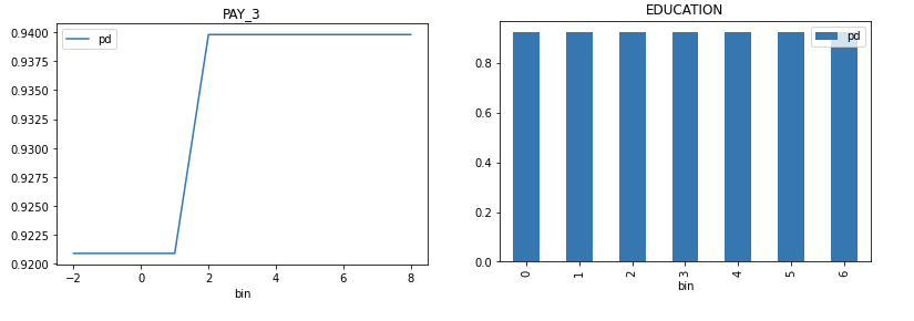
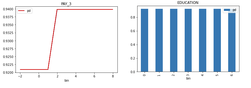
Partial Dependence/Individual Conditional Expectations (PD/ICE) Explainer

Partial dependence plot (PDP) portrays the average prediction behavior of the model across the domain of an input variable along with +/- 1 standard deviation bands. Individual Conditional Expectations plot (ICE) displays the prediction behavior for an individual row of data when an input variable is toggled across its domain.

Explainer parameters:

• sample_size

  • Sample size (default is 100 000).

• max_features

  • Partial Dependence Plot number of features (to see all features used by model set to -1).

• features

  • Partial Dependence Plot feature list.

• grid_resolution

  • Partial Dependence Plot observations per bin (number of equally spaced points used to create bins).

• oor_grid_resolution

  • Partial Dependence Plot number of out of range bins.

• center

  • Center Partial Dependence Plot using ICE centered at 0.

• sort_bins

  • Ensure bin values sorting.

• quantile-bin-grid-resolution

  • Partial Dependence Plot quantile binning (total quantile points used to create bins).

• quantile-bins

  • Per-feature quantile binning.

  • Example: if choosing features F1 and F2, this parameter is {"F1": 2,"F2": 5}. Note, you can set all features to use the same quantile binning with the “Partial Dependence Plot quantile binning” parameter and then adjust the quantile binning for a subset of PDP features with this parameter.

• histograms

  • Enable or disable histograms.

• numcat_num_chart

  • Unique feature values count driven Partial Dependence Plot binning and chart selection.

• numcat_threshold

  • Threshold for Partial Dependence Plot binning and chart selection (<= threshold categorical, > threshold numeric).

Explainer result directory description:

explainer_h2o_sonar_explainers_pd_ice_explainer_PdIceExplainer_ee264725-cdab-476c-bad5-02cf778e1c1e
├── global_partial_dependence
│   ├── application_json
│   │   ├── explanation.json
│   │   ├── pd_feature_0_class_0.json
│   │   ├── pd_feature_1_class_0.json
│   │   ├── pd_feature_2_class_0.json
│   │   ├── pd_feature_3_class_0.json
│   │   ├── pd_feature_4_class_0.json
│   │   ├── pd_feature_5_class_0.json
│   │   ├── pd_feature_6_class_0.json
│   │   ├── pd_feature_7_class_0.json
│   │   ├── pd_feature_8_class_0.json
│   │   └── pd_feature_9_class_0.json
│   └── application_json.meta
├── local_individual_conditional_explanation
│   ├── application_vnd_h2oai_json_datatable_jay
│   │   ├── explanation.json
│   │   ├── ice_feature_0_class_0.jay
│   │   ├── ice_feature_1_class_0.jay
│   │   ├── ice_feature_2_class_0.jay
│   │   ├── ice_feature_3_class_0.jay
│   │   ├── ice_feature_4_class_0.jay
│   │   ├── ice_feature_5_class_0.jay
│   │   ├── ice_feature_6_class_0.jay
│   │   ├── ice_feature_7_class_0.jay
│   │   ├── ice_feature_8_class_0.jay
│   │   ├── ice_feature_9_class_0.jay
│   │   └── y_hat.jay
│   └── application_vnd_h2oai_json_datatable_jay.meta
├── log
│   └── explainer_run_ee264725-cdab-476c-bad5-02cf778e1c1e.log
├── result_descriptor.json
└── work
    ├── h2o_sonar-ice-dai-model-10.jay
    ├── h2o_sonar-ice-dai-model-1.jay
    ├── h2o_sonar-ice-dai-model-2.jay
    ├── h2o_sonar-ice-dai-model-3.jay
    ├── h2o_sonar-ice-dai-model-4.jay
    ├── h2o_sonar-ice-dai-model-5.jay
    ├── h2o_sonar-ice-dai-model-6.jay
    ├── h2o_sonar-ice-dai-model-7.jay
    ├── h2o_sonar-ice-dai-model-8.jay
    ├── h2o_sonar-ice-dai-model-9.jay
    ├── h2o_sonar-ice-dai-model.json
    ├── h2o_sonar-pd-dai-model.json
    └── mli_dataset_y_hat.jay

• explainer_.../work/

  • Data artifacts used to calculate PD and ICE.

Explanations created by the explainer:

• global_partial_dependence

  • Per-feature partial dependence explanation in JSon format.

• local_individual_conditional_explanation

  • Per-feature individual conditional expectation explanation in JSon and datatable format.

PD/ICE explainer binning:

• Integer feature:

  • bins in numeric mode:

    • bins are integers

    • (at most) grid_resolution integer values in between minimum and maximum of feature values

    • bin values are created as evenly as possible

    • minimum and maximum is included in bins (if grid_resolution is bigger or equal to 2)

  • bins in categorical mode:

    • bins are integers

    • top grid_resolution values from feature values ordered by frequency (int values are converted to strings and most frequent values are used as bins)

  • quantile bins in numeric mode:

    • bins are integers

    • bin values are created with the aim that there will be the same number of observations per bin

    • q-quantile used to created q bins where q is specified by PD parameter

  • quantile bins in categorical mode:

    • not supported

• Float feature:

  • bins in numeric mode:

    • bins are floats

    • grid_resolution float values in between minimum and maximum of feature

      values

    • bin values are created as evenly as possible

    • minimum and maximum is included in bins (if grid_resolution is bigger or equal to 2)

  • bins in categorical mode:

    • bins are floats

    • top grid_resolution values from feature values ordered by frequency (float values are converted to strings and most frequent values are used as bins)

  • quantile bins in numeric mode:

    • bins are floats

    • bin values are created with the aim that there will be the same number of observations per bin

    • q-quantile used to created q bins where q is specified by PD parameter

  • quantile bins in categorical mode:

    • not supported

• String feature:

  • bins in numeric mode:

    • not supported

  • bins in categorical mode:

    • bins are strings

    • top grid_resolution values from feature values ordered by frequency

  • quantile bins:

    • not supported

• Date/datetime feature:

  • bins in numeric mode:

    • bins are dates

    • grid_resolution date values in between minimum and maximum of feature values

    • bin values are created as evenly as possible:

      1. dates are parsed and converted to epoch timestamps i.e integers

      2. bins are created as in case of numeric integer binning

      3. integer bins are converted back to original date format

    • minimum and maximum is included in bins (if grid_resolution is bigger or equal to 2)

  • bins in categorical mode:

    • bins are dates

    • top grid_resolution values from feature values ordered by frequency (dates are handled as opaque strings and most frequent values are used as bins)

  • quantile bins:

    • not supported

PD/ICE explainer out of range binning:

• Integer feature:

  • OOR bins in numeric mode:

    • OOR bins are integers

    • (at most) oor_grid_resolution integer values are added below minimum and above maximum

    • bin values are created by adding/substracting rounded standard deviation (of feature values) above and below maximum and minimum oor_grid_resolution times

      • 1 used used if rounded standard deviation would be 0

    • if feature is of unsigned integer type, then bins below 0 are not created

      • if rounded standard deviation and/or oor_grid_resolution is so high that it would cause lower OOR bins to be negative numbers, then standard deviation of size 1 is tried instead

  • OOR bins in categorical mode:

    • same as numeric mode

• Float feature:

  • OOR bins in numeric mode:

    • OOR bins are floats

    • oor_grid_resolution float values are added below minimum and above maximum

    • bin values are created by adding/substracting standard deviation (of feature values) above and below maximum and minimum oor_grid_resolution times

  • OOR bins in categorical mode:

    • same as numeric mode

• String feature:

  • bins in numeric mode:

    • not supported

  • bins in categorical mode:

    • OOR bins are strings

    • value UNSEEN is added as OOR bin

• Date feature:

  • bins in numeric mode:

    • not supported

  • bins in categorical mode:

    • OOR bins are strings

    • value UNSEEN is added as OOR bin

See also:

• Partial dependence / Individual Conditional Expectation (PD/ICE) Explainer Demo

• Interpretation Directory Structure

• Explainer Parameters

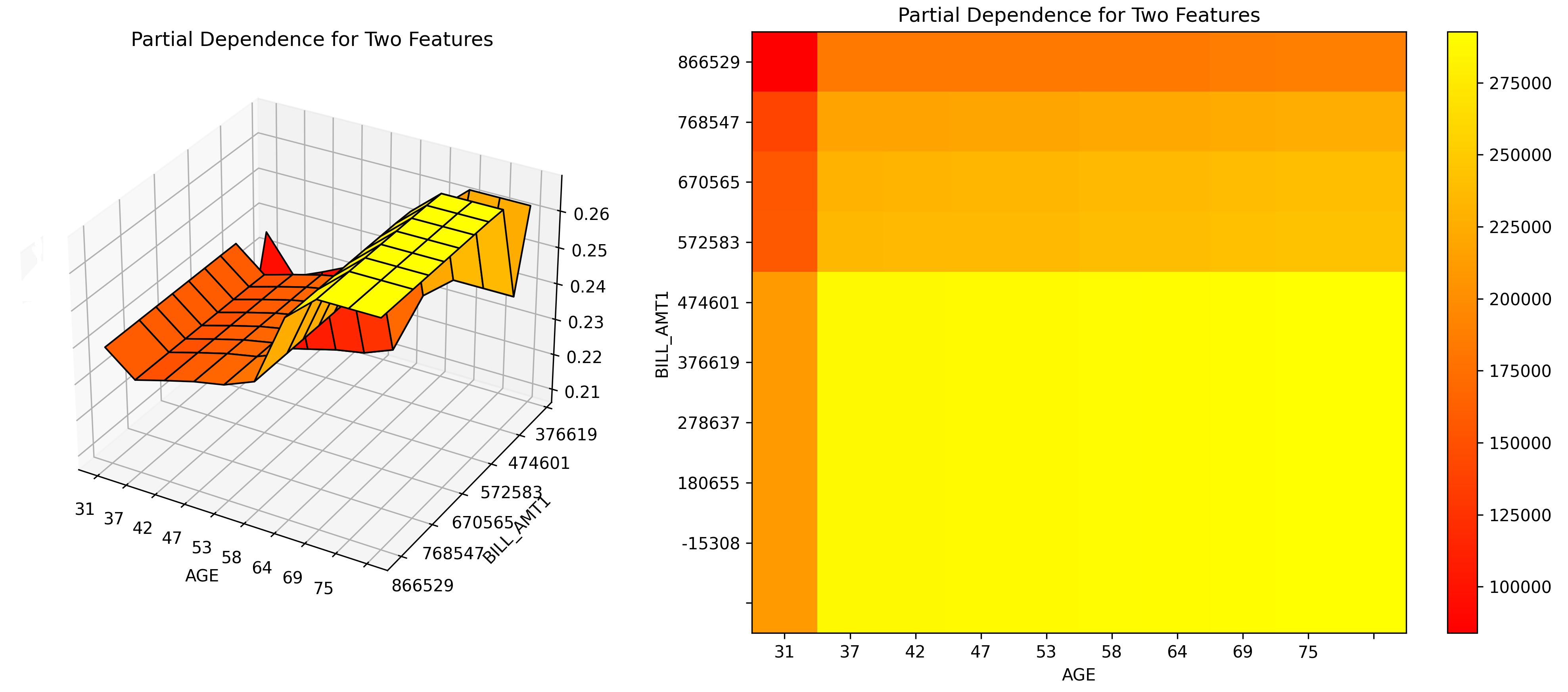
Partial Dependence for 2 Features Explainer

Partial dependence for 2 features portrays the average prediction behavior of a model across the domains of two input variables i.e. interaction of feature tuples with the prediction. While PD for one feature produces 2D plot, PD for two features produces 3D plots. This explainer plots PD for two features using heatmap, contour 3D or surface 3D.

Explainer parameters:

• sample_size

  • Sample size (default is 100 000).

• max_features

  • Partial Dependence Plot number of features (to see all features used by model set to -1).

• features

  • Partial Dependence Plot feature list.

• grid_resolution

  • Partial Dependence Plot observations per bin (number of equally spaced points used to create bins).

• oor_grid_resolution

  • Partial Dependence Plot number of out of range bins.

• quantile-bin-grid-resolution

  • Partial Dependence Plot quantile binning (total quantile points used to create bins).

• plot_type

  • Plot type to be used for Partial Dependence rendering - heatmap, contour-3d or surface-3d.

Explainer result directory description:

explainer_h2o_sonar_explainers_pd_2_features_explainer_PdFor2FeaturesExplainer_f710d221-64dc-4dc3-8e1f-2922d5a32cab
├── global_3d_data
│   ├── application_json
│   │   ├── data3d_feature_0_class_0.json
│   │   ├── data3d_feature_1_class_0.json
│   │   ├── data3d_feature_2_class_0.json
│   │   ├── data3d_feature_3_class_0.json
│   │   ├── data3d_feature_4_class_0.json
│   │   ├── data3d_feature_5_class_0.json
│   │   └── explanation.json
│   ├── application_json.meta
│   ├── application_vnd_h2oai_json_csv
│   │   ├── data3d_feature_0_class_0.csv
│   │   ├── data3d_feature_1_class_0.csv
│   │   ├── data3d_feature_2_class_0.csv
│   │   ├── data3d_feature_3_class_0.csv
│   │   ├── data3d_feature_4_class_0.csv
│   │   ├── data3d_feature_5_class_0.csv
│   │   └── explanation.json
│   └── application_vnd_h2oai_json_csv.meta
├── global_html_fragment
│   ├── text_html
│   │   ├── explanation.html
│   │   ├── image-0.png
│   │   ├── image-1.png
│   │   ├── image-2.png
│   │   ├── image-3.png
│   │   ├── image-4.png
│   │   └── image-5.png
│   └── text_html.meta
├── global_report
│   ├── text_markdown
│   │   ├── explanation.md
│   │   ├── image-0.png
│   │   ├── image-1.png
│   │   ├── image-2.png
│   │   ├── image-3.png
│   │   ├── image-4.png
│   │   └── image-5.png
│   └── text_markdown.meta
├── log
│   └── explainer_run_f710d221-64dc-4dc3-8e1f-2922d5a32cab.log
├── model_problems
│   └── problems_and_actions.json
├── result_descriptor.json
└── work
    ├── ...
    └── report.md

• explainer_.../work/

  • Data artifacts used to calculate the PD for 2 features.

Explanations created by the explainer:

• global_3d_data

  • Per-feature tuple partial dependence explanation in JSon and CSV format.

• global_report

  • Per-feature tuple partial dependence report in Markdown format.

• global_html_fragment

  • Per-feature tuple partial dependence report as HTML snippet.

See also:

• Partial Dependence for 2 Features Explainer Demo

• Interpretation Directory Structure

• Explainer Parameters

Residual Partial Dependence/Individual Conditional Expectations (PD/ICE) Explainer

The residual partial dependence plot (PDP) indicates which variables interact most with the error. Residuals are differences between observed and predicted values - the square of the difference between observed and predicted values is used. The residual partial dependence is created using normal partial dependence algorithm, while instead of prediction is used the residual. Individual Conditional Expectations plot (ICE) displays the interaction with error for an individual row of data when an input variable is toggled across its domain.

Explainer parameters:

• sample_size

  • Sample size (default is 100 000).

• max_features

  • Residual Partial Dependence Plot number of features (to see all features used by model set to -1).

• features

  • Residual Partial Dependence Plot feature list.

• grid_resolution

  • Residual Partial Dependence Plot observations per bin (number of equally spaced points used to create bins).

• oor_grid_resolution

  • Residual Partial Dependence Plot number of out of range bins.

• center

  • Center Partial Dependence Plot using ICE centered at 0.

• sort_bins

  • Ensure bin values sorting.

• quantile-bin-grid-resolution

  • Residual Partial Dependence Plot quantile binning (total quantile points used to create bins).

• quantile-bins

  • Per-feature quantile binning.

  • Example: if choosing features F1 and F2, this parameter is {"F1": 2,"F2": 5}. Note, you can set all features to use the same quantile binning with the “Partial Dependence Plot quantile binning” parameter and then adjust the quantile binning for a subset of PDP features with this parameter.

• histograms

  • Enable or disable histograms.

• numcat_num_chart

  • Unique feature values count driven Partial Dependence Plot binning and chart selection.

• numcat_threshold

  • Threshold for Partial Dependence Plot binning and chart selection (<= threshold categorical, > threshold numeric).

Explainer result directory description:

tree explainer_h2o_sonar_explainers_residual_pd_ice_explainer_ResidualPdIceExplainer_40eb4da9-4a68-4782-9a70-22c6f7984846
explainer_h2o_sonar_explainers_residual_pd_ice_explainer_ResidualPdIceExplainer_40eb4da9-4a68-4782-9a70-22c6f7984846
├── global_html_fragment
│   ├── text_html
│   │   ├── explanation.html
│   │   ├── pd-class-1-feature-10.png
│   │   ├── pd-class-1-feature-1.png
│   │   ├── pd-class-1-feature-2.png
│   │   ├── pd-class-1-feature-3.png
│   │   ├── pd-class-1-feature-4.png
│   │   ├── pd-class-1-feature-5.png
│   │   ├── pd-class-1-feature-6.png
│   │   ├── pd-class-1-feature-7.png
│   │   ├── pd-class-1-feature-8.png
│   │   └── pd-class-1-feature-9.png
│   └── text_html.meta
├── global_partial_dependence
│   ├── application_json
│   │   ├── explanation.json
│   │   ├── pd_feature_0_class_0.json
│   │   ├── pd_feature_1_class_0.json
│   │   ├── pd_feature_2_class_0.json
│   │   ├── pd_feature_3_class_0.json
│   │   ├── pd_feature_4_class_0.json
│   │   ├── pd_feature_5_class_0.json
│   │   ├── pd_feature_6_class_0.json
│   │   ├── pd_feature_7_class_0.json
│   │   ├── pd_feature_8_class_0.json
│   │   └── pd_feature_9_class_0.json
│   └── application_json.meta
├── local_individual_conditional_explanation
│   ├── application_vnd_h2oai_json_datatable_jay
│   │   ├── explanation.json
│   │   ├── ice_feature_0_class_0.jay
│   │   ├── ice_feature_1_class_0.jay
│   │   ├── ice_feature_2_class_0.jay
│   │   ├── ice_feature_3_class_0.jay
│   │   ├── ice_feature_4_class_0.jay
│   │   ├── ice_feature_5_class_0.jay
│   │   ├── ice_feature_6_class_0.jay
│   │   ├── ice_feature_7_class_0.jay
│   │   ├── ice_feature_8_class_0.jay
│   │   ├── ice_feature_9_class_0.jay
│   │   └── y_hat.jay
│   └── application_vnd_h2oai_json_datatable_jay.meta
├── log
│   └── explainer_run_40eb4da9-4a68-4782-9a70-22c6f7984846.log
├── model_problems
│   └── problems_and_actions.json
├── result_descriptor.json
└── work
    ├── h2o_sonar-ice-dai-model-10.jay
    ├── h2o_sonar-ice-dai-model-1.jay
    ├── h2o_sonar-ice-dai-model-2.jay
    ├── h2o_sonar-ice-dai-model-3.jay
    ├── h2o_sonar-ice-dai-model-4.jay
    ├── h2o_sonar-ice-dai-model-5.jay
    ├── h2o_sonar-ice-dai-model-6.jay
    ├── h2o_sonar-ice-dai-model-7.jay
    ├── h2o_sonar-ice-dai-model-8.jay
    ├── h2o_sonar-ice-dai-model-9.jay
    ├── h2o_sonar-ice-dai-model.json
    ├── h2o_sonar-pd-dai-model.json
    └── mli_dataset_y_hat.jay

• explainer_.../work/

  • Data artifacts used to calculate residual PD and ICE.

Explanations created by the explainer:

• global_partial_dependence

  • Per-feature residual partial dependence explanation in JSon format.

• local_individual_conditional_explanation

  • Per-feature residual individual conditional expectation explanation in JSon and datatable format.

Residual PD/ICE explainer binning is the same as in case of Partial Dependence/Individual Conditional Expectations (PD/ICE) Explainer.

Problems reported by the explainer:

• Highest interaction between a feature and the error

  • The explainer reports a column with highest interaction with the error. This column (feature) should be investigated to determine whether it indicates a problem with the model.

  • Problem severity: MEDIUM.

See also:

• Residual Partial dependence / Individual Conditional Expectation (PD/ICE) Explainer Demo

• Interpretation Directory Structure

• Explainer Parameters

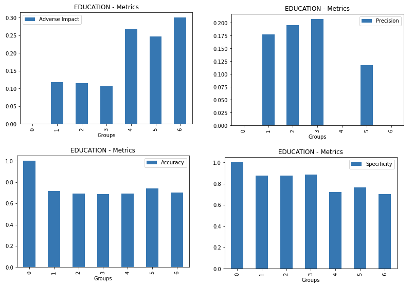
Disparate Impact Analysis (DIA) Explainer

Disparate Impact Analysis (DIA) is a technique that is used to evaluate fairness. Bias can be introduced to models during the process of collecting, processing, and labeling data as a result, it is important to determine whether a model is harming certain users by making a significant number of biased decisions. DIA typically works by comparing aggregate measurements of unprivileged groups to a privileged group. For instance, the proportion of the unprivileged group that receives the potentially harmful outcome is divided by the proportion of the privileged group that receives the same outcome - the resulting proportion is then used to determine whether the model is biased.

Explainer parameters:

• dia_cols

  • List of features for which to compute DIA.

• cut_off

  • Cut off.

• maximize_metric

  • Maximize metric - one of F1, F05, F2, MCC (default is F1).

• sample_size

  • Sample size (default is 100 000).

• max_cardinality

  • Max cardinality for categorical variables (default is 10).

• min_cardinality

  • Min cardinality for categorical variables (default is 2).

• num_card

  • Max cardinality for numeric variables to be considered categorical (default is 25).

Explainer result directory description:

explainer_h2o_sonar_explainers_dia_explainer_DiaExplainer_f1600947-05bc-4ae0-a396-d69dfca9d7c7
├── global_disparate_impact_analysis
│   ├── text_plain
│   │   └── explanation.txt
│   └── text_plain.meta
├── log
│   └── explainer_run_f1600947-05bc-4ae0-a396-d69dfca9d7c7.log
├── result_descriptor.json
└── work
    ├── dia_entity.json
    ├── EDUCATION
    │   ├── 0
    │   │   ├── cm.jay
    │   │   ├── disparity.jay
    │   │   ├── me_smd.jay
    │   │   └── parity.jay
    │   ├── 1
    │   │   ├── cm.jay
    │   │   ├── disparity.jay
    │   │   ├── me_smd.jay
    │   │   └── parity.jay
    │   ├── 2
    │   │   ├── cm.jay
    │   │   ├── disparity.jay
    │   │   ├── me_smd.jay
    │   │   └── parity.jay
    │   ├── 3
    │   │   ├── cm.jay
    │   │   ├── disparity.jay
    │   │   ├── me_smd.jay
    │   │   └── parity.jay
    │   ├── 4
    │   │   ├── cm.jay
    │   │   ├── disparity.jay
    │   │   ├── me_smd.jay
    │   │   └── parity.jay
    │   ├── 5
    │   │   ├── cm.jay
    │   │   ├── disparity.jay
    │   │   ├── me_smd.jay
    │   │   └── parity.jay
    │   ├── 6
    │   │   ├── cm.jay
    │   │   ├── disparity.jay
    │   │   ├── me_smd.jay
    │   │   └── parity.jay
    │   └── metrics.jay
    ├── MARRIAGE
    ...
    └── SEX
        ├── 0
        │   ├── cm.jay
        │   ├── disparity.jay
        │   ├── me_smd.jay
        │   └── parity.jay
        ├── 1
        │   ├── cm.jay
        │   ├── disparity.jay
        │   ├── me_smd.jay
        │   └── parity.jay
        └── metrics.jay

• explainer_.../work/<feature name/

  • Per feature directory with Disparate Impact Analysis metrics family - like disparity, parity, SMD and CM - for each feature value (group) in datatable format.

Explanations created by the explainer:

• global_disparate_impact_analysis

  • Disparate impact analysis explanation.

See also:

• Disparate Impact Analysis (DIA) Explainer Demo

• Interpretation Directory Structure

• Explainer Parameters

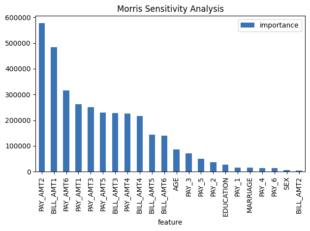
Morris sensitivity analysis Explainer

Morris sensitivity analysis (SA) explainer provides Morris sensitivity analysis based feature importance which is a measure of the contribution of an input variable to the overall predictions of the model. In applied statistics, the Morris method for global sensitivity analysis is a so-called one-step-at-a-time method (OAT), meaning that in each run only one input parameter is given a new value. This explainer is based based on InterpretML library - see interpret.ml.

Package requirements:

• install interpret library as it is not installed with H2O Eval Studio by default:

pip install interpret

Explainer parameters:

• leakage_warning_threshold

  • Threshold for showing potential data leakage in the most important feature. Data leakage occurs when a feature influences the target column too much. High feature importance value means that the model you trained with this dataset will not be predicting the target based on all features but rather on just one. More about feature data leakage (also target leakage) at Target leakage H2O.ai Wiki.

Explainer result directory description:

explainer_h2o_sonar_explainers_morris_sa_explainer_MorrisSensitivityAnalysisExplainer_f4da0294-8c2b-4195-a567-bd4b65a01227
├── global_feature_importance
│   ├── application_json
│   │   ├── explanation.json
│   │   └── feature_importance_class_0.json
│   ├── application_json.meta
│   ├── application_vnd_h2oai_json_datatable_jay
│   │   ├── explanation.json
│   │   └── feature_importance_class_0.jay
│   └── application_vnd_h2oai_json_datatable_jay.meta
├── global_html_fragment
│   ├── text_html
│   │   ├── explanation.html
│   │   └── fi-class-0.png
│   └── text_html.meta
├── log
│   └── explainer_run_f4da0294-8c2b-4195-a567-bd4b65a01227.log
├── result_descriptor.json
└── work

Explanations created by the explainer:

• global_feature_importance

  • Feature interactions in JSon format.

• global_html_fragment

  • Feature interactions in HTML format.

Problems reported by the explainer:

• Potential feature importance leak

  • The explainer reports a column with potential feature importance leak. Such column should be investigated and in case of the leak either removed from the dataset or weighted down in the model training process.

  • Problem severity: HIGH.

See also:

• Morris Sensitivity Analysis Explainer Demo

• Interpretation Directory Structure

• Explainer Parameters

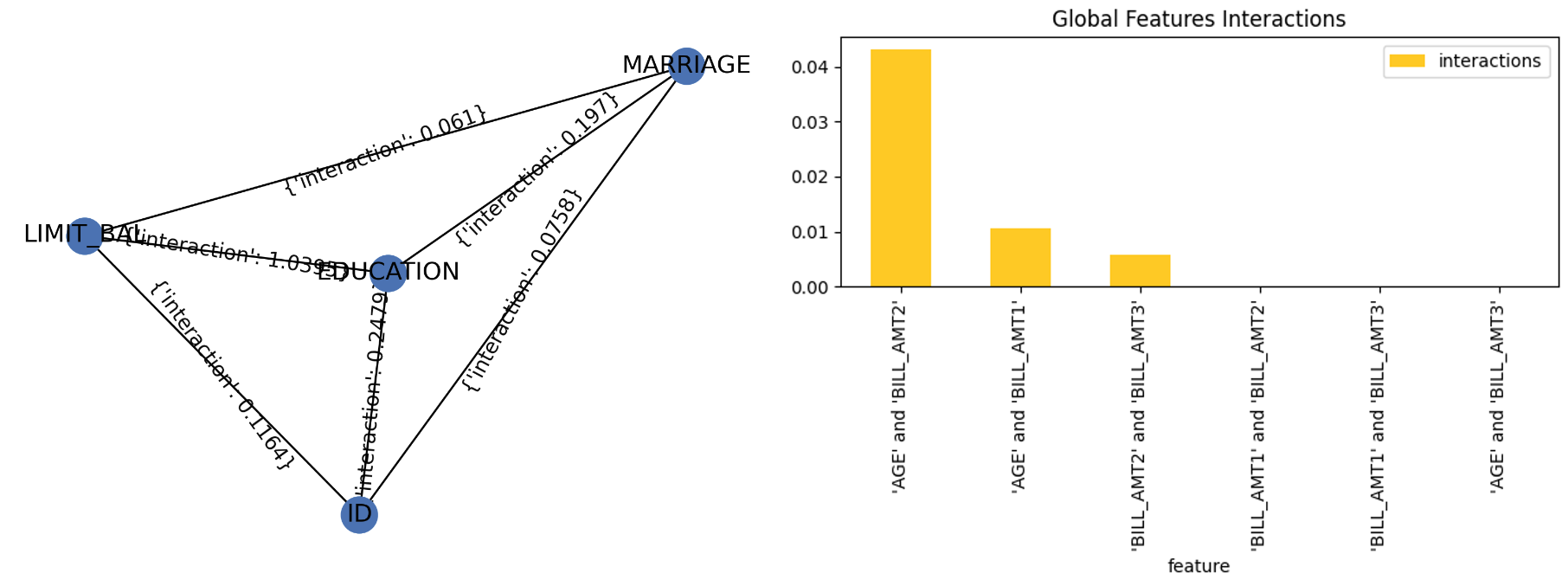
Friedman’s H-statistic Explainer

The explainer provides implementation of Friedman’s H-statistic feature interactions. The statistic is 0 when there is no interaction at all and 1 if all the variance of the predict function is explained by a sum of the partial dependence functions. More information about Friedman’s H-Statistic method is available at Theory: Friedman’s H-statistic.

Explainer parameters:

• features_number

  • Maximum number of features for which to calculate Friedman’s H-statistic (must be at least 2).

• features

  • List of features for which to calculate Friedman’s H-statistic (must be at least 2, overrides features_number).

• grid_resolution

  • Friedman’s H-statistic observations per bin (number of equally spaced points used to create bins).

Explainer result directory description:

explainer_h2o_sonar_explainers_friedman_h_statistic_explainer_FriedmanHStatisticExplainer_579aa93f-4f80-446f-ba21-815304ccee9c
├── global_feature_importance
│   ├── application_json
│   │   ├── explanation.json
│   │   └── feature_importance_class_0.json
│   ├── application_json.meta
│   ├── application_vnd_h2oai_json_csv
│   │   ├── explanation.json
│   │   └── feature_importance_class_0.csv
│   ├── application_vnd_h2oai_json_csv.meta
│   ├── application_vnd_h2oai_json_datatable_jay
│   │   ├── explanation.json
│   │   └── feature_importance_class_0.jay
│   └── application_vnd_h2oai_json_datatable_jay.meta
├── global_html_fragment
│   ├── text_html
│   │   ├── explanation.html
│   │   └── fi-class-0.png
│   └── text_html.meta
├── global_report
│   ├── text_markdown
│   │   ├── explanation.md
│   │   └── image.png
│   └── text_markdown.meta
├── log
│   └── explainer_run_579aa93f-4f80-446f-ba21-815304ccee9c.log
├── result_descriptor.json
└── work
    ├── image.png
    └── report.md

Explanations created by the explainer:

• global_feature_importance

  • Feature interactions in JSon, CSV and datatable formats.

• global_html_fragment

  • Feature interactions in HTML format.

• global_report

  • Feature interactions in Markdown format.

See also:

• Friedman H-statistic Explainer Demo

• Interpretation Directory Structure

• Explainer Parameters

Dataset and Model Insights Explainer

The explainer checks the dataset and model for various issues. For example, it provides problems and actions for missing values in the target column and a low number of unique values across columns of a dataset.

Explainer result directory description:

explainer_h2o_sonar_explainers_dataset_and_model_insights_DatasetAndModelInsights_e222f392-9a55-41fb-ab51-d45cc6bd35db/
├── global_text_explanation
│   ├── text_plain
│   │   └── explanation.txt
│   └── text_plain.meta
├── log
│   └── explainer_run_e222f392-9a55-41fb-ab51-d45cc6bd35db.log
├── model_problems
│   └── problems_and_actions.json
├── result_descriptor.json
└── work

Problems reported by the explainer:

• Missing values in the target column

  • The explainer reports missing values in the target column. Rows with the missing values in the target column should be removed from the dataset.

  • Problem severity: LOW - HIGH (based on the number of impacted columns).

• Features with potentially insufficient number of unique values

  • The explainer reports columns with 1 unique value only. Such columns should be either removed from the dataset or its missing values (if any) replaced with valid values.

  • Problem severity: LOW - HIGH (based on the number of impacted columns).

See also:

• Dataset and Model Insights Explainer Demo

• Interpretation Directory Structure

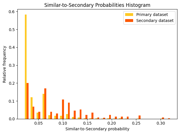
Adversarial Similarity Explainer

This explainer is based on the adversarial similarity H2O Model Validation test.

Adversarial similarity refers to a validation test that assists in observing feature distribution of two different datasets can indicate similarity or dissimilarity. An adversarial similarity test can be performed rather than going over all the features individually to observe the differences. During an adversarial similarity test, decision tree algorithms are leveraged to find similar or dissimilar rows between the train dataset and any dataset with the same train columns.

Explainer parameters:

• worker_connection_key

  • Optional connection ID of the Driverless AI worker configured in the H2O Eval Studio configuration. Supported are Driverless AI servers hosted by H2O AIEM or H2O Enterprise Steam, or Driverless AI servers that use username and password authentication.

• shapley_values

  • Determines whether to compute Shapley values for the model used to analyze the similarity between the Primary and Secondary Dataset. Test uses the generated Shapley values to create an array of visual metrics that provide valuable insights into the contribution of individual features to the overall model performance.

• drop_cols

  • Defines the columns to drop during model training.

The explainer can be run using the Python API as follows:

# configure Driverless AI server to serve as a host of artifacts (datasets, models) and/or worker
DAI_CONNECTION = h2o_sonar_config.ConnectionConfig(
   key="local-driverless-ai-server",  # ID is generated from the connection name (NCName)
   connection_type=h2o_sonar_config.ConnectionConfigType.DRIVERLESS_AI_AIEM.name,
   name="My H2O AIEM hosted Driverless AI ",
   description="Driverless AI server hosted by H2O Enterprise AIEM.",
   server_url="https://enginemanager.cloud.h2o.ai/",
   server_id="new-dai-engine-42",
   environment_url="https://cloud.h2o.ai",
   username="firstname.lastname@h2o.ai",
   token=os.getenv(KEY_AIEM_REFRESH_TOKEN_CLOUD),
   token_use_type=h2o_sonar_config.TokenUseType.REFRESH_TOKEN.name,
)
# add the connection to the H2O Eval Studio configuration
h2o_sonar_config.config.add_connection(DAI_CONNECTION)

# run the explainer (model and datasets provided as handles as they are hosted by the Driverless AI server)
interpretation = interpret.run_interpretation(
   model=f"resource:connection:{DAI_CONNECTION.key}:key:7965e2ea-f898-11ed-b979-106530ed5ceb",
   dataset=f"resource:connection:{DAI_CONNECTION.key}:key:8965e2ea-f898-11ed-b979-106530ed5ceb",
   testset=f"resource:connection:{DAI_CONNECTION.key}:key:9965e2ea-f898-11ed-b979-106530ed5ceb",
   target_col="Weekly_Sales",
   explainers=[
      commons.ExplainerToRun(
            explainer_id=AdversarialSimilarityExplainer.explainer_id(),
            params={
               "worker_connection_key": DAI_CONNECTION.key,
               "shapley_values": False,
            },
      )
   ],
   results_location="./h2o-sonar-results",
)

The explainer can be run using the command line interface (CLI) as follows:

h2o-sonar run interpretation
--explainers h2o_sonar.explainers.adversarial_similarity_explainer.AdversarialSimilarityExplainer
--explainers-pars '{
   "h2o_sonar.explainers.adversarial_similarity_explainer.AdversarialSimilarityExplainer": {
      "worker_connection_key": "local-driverless-ai-server",
      "shapley_values": false,
   }
}'
--model "resource:connection:local-driverless-ai-server:key:7965e2ea-f898-11ed-b979-106530ed5ceb"
--dataset "resource:connection:local-driverless-ai-server:key:695f5d5e-f898-11ed-b979-106530ed5ceb"
--testset "resource:connection:local-driverless-ai-server:key:695df75c-f898-11ed-b979-106530ed5ceb"
--target-col "Weekly_Sales"
--results-location "./h2o-sonar-results"
--config-path "./h2o-sonar-config.json"
--encryption-key "secret-key-to-decrypt-encrypted-config-fields"

Explainer result directory description:

explainer_h2o_sonar_explainers_adversarial_similarity_explainer_AdversarialSimilarityExplainer_d473b5c0-02a3-4971-905a-adb9841a0958
├── global_grouped_bar_chart
│   ├── application_vnd_h2oai_json_datatable_jay
│   │   ├── explanation.json
│   │   └── feature_importance_class_0.jay
│   └── application_vnd_h2oai_json_datatable_jay.meta
├── global_html_fragment
│   ├── text_html
│   │   ├── explanation.html
│   │   └── fi-class-0.png
│   └── text_html.meta
├── global_work_dir_archive
│   ├── application_zip
│   │   └── explanation.zip
│   └── application_zip.meta
├── log
│   └── explainer_run_d473b5c0-02a3-4971-905a-adb9841a0958.log
├── model_problems
│   └── problems_and_actions.json
├── result_descriptor.json
└── work

Explanations created by the explainer:

• global_grouped_bar_chart

  • Similar-to-secondary probabilities histogram in the datatable format.

• global_html_fragment

  • Adversarial similarity in the HTML format.

• global_work_dir_archive

  • All explanations created by the explainer stored in a ZIP archive.

See also:

• H2O Model Validation documentation of the Adversarial Similarity explainer

• H2O Eval Studio Model Validation Explainers

• Interpretation Directory Structure

• Library Configuration

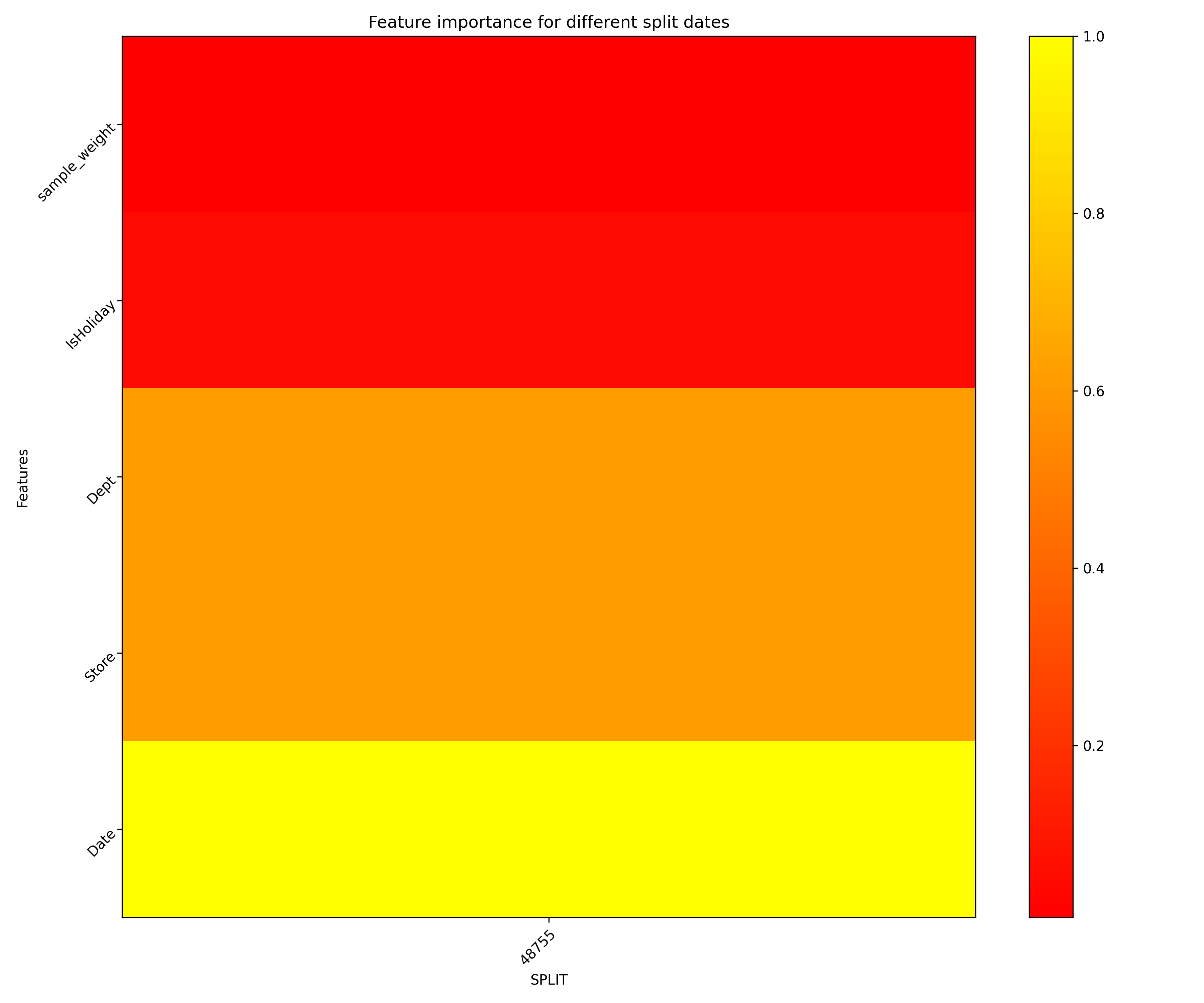
Backtesting Explainer

This explainer is based on the backtesting H2O Model Validation test.

A backtesting test enables you to assess the robustness of a model using the existing historical training data through a series of iterative training where training data is used from its recent to oldest collected values.

Explainer performs a backtesting test by fitting a predictive model with a training dataset to later assess the model with a separate test dataset where the test dataset does not overlap with the training data. Frequently, the training data is collected over time and has an explicit time dimension. In such cases, utilizing the most recent dataset points for the model test dataset is common practice, as it better mimics a real model application.

By applying a backtesting test to a model, we can refit the model multiple times, where every time, we use shorter time spans of the training data while using a portion of that data as test data. As a result, the test dataset is replaced with a series of values over time.

A backtesting test enables you to:

• Understand the variance of the model accuracy

• Understand and visualize how the model accuracy develops over time

• Identify potential reasons for any performance issues with the modeling approach in the past (for example, problems around data collection)

Each iteration during backtesting, the model is fully refitted, which includes a rerun of feature engineering and feature selection. Not entirely refitting during each iteration results in an incorrect backtesting outcome because the next iteration would have selected features based on the entire data. An incorrect backtesting outcome also leads to data leakage where information from the future is explicitly or implicitly reflected in the current variables.

Explainer parameters:

• worker_connection_key

  • The connection ID of the Driverless AI worker configured in the H2O Eval Studio configuration. Supported are Driverless AI servers hosted by H2O AIEM or H2O Enterprise Steam, or Driverless AI servers that use username and password authentication.

• time_col

  • Defines the time column in the primary dataset that the explainer utilizes to split the primary dataset (training dataset) during the backtesting test.

• split_type

  • Split type - either ‘auto’ (explainer determines the split dates, which create the backtesting experiments) or ‘custom’ (you determine the split dates, which create the backtesting experiments).

• number_of_splits

  • Defines the number of dates (splits) the explainer utilizes for the dataset splitting and model refitting process during the validation test. The explainer sets the specified number of dates in the past while being equally apart from one another to generate appropriate dataset splits.

• number_of_forecast_periods

  • Number of the forest periods.

• forecast_period_unit

  • Forecast period unit.

• number_of_training_periods

  • Number of training periods.

• training_period_unit

  • Training period unit.

• custom_dates

  • Custom dates.

• plot_type

  • Plot type - one of heatmap, contour-3d or surface-3d.

The explainer can be run using the Python API as follows:

# configure Driverless AI server to serve as a host of artifacts (datasets, models) and/or worker
DAI_CONNECTION = h2o_sonar_config.ConnectionConfig(
   key="local-driverless-ai-server",  # ID is generated from the connection name (NCName)
   connection_type=h2o_sonar_config.ConnectionConfigType.DRIVERLESS_AI_AIEM.name,
   name="My H2O AIEM hosted Driverless AI ",
   description="Driverless AI server hosted by H2O Enterprise AIEM.",
   server_url="https://enginemanager.cloud.h2o.ai/",
   server_id="new-dai-engine-42",
   environment_url="https://cloud.h2o.ai",
   username="firstname.lastname@h2o.ai",
   token=os.getenv(KEY_AIEM_REFRESH_TOKEN_CLOUD),
   token_use_type=h2o_sonar_config.TokenUseType.REFRESH_TOKEN.name,
)
# add the connection to the H2O Eval Studio configuration
h2o_sonar_config.config.add_connection(DAI_CONNECTION)

# run the explainer (model and datasets provided as handles as they are hosted by the Driverless AI server)
interpretation = interpret.run_interpretation(
   model=f"resource:connection:{DAI_CONNECTION.key}:key:7965e2ea-f898-11ed-b979-106530ed5ceb",
   dataset=f"resource:connection:{DAI_CONNECTION.key}:key:8965e2ea-f898-11ed-b979-106530ed5ceb",
   target_col="Weekly_Sales",
   explainers=[
      commons.ExplainerToRun(
            explainer_id=BacktestingExplainer.explainer_id(),
            params={
               "worker_connection_key": DAI_CONNECTION.key,
               "time_col": "Date",
            },
      )
   ],
   results_location="./h2o-sonar-results",
)

The explainer can be run using the command line interface (CLI) as follows:

h2o-sonar run interpretation
--explainers h2o_sonar.explainers.backtesting_explainer.BacktestingExplainer
--explainers-pars '{
   "h2o_sonar.explainers.backtesting_explainer.BacktestingExplainer": {
      "worker_connection_key": "local-driverless-ai-server",
      "shapley_values": false,
   }
}'
--model "resource:connection:local-driverless-ai-server:key:7965e2ea-f898-11ed-b979-106530ed5ceb"
--dataset "resource:connection:local-driverless-ai-server:key:695f5d5e-f898-11ed-b979-106530ed5ceb"
--target-col "Weekly_Sales"
--results-location "./h2o-sonar-results"
--config-path "./h2o-sonar-config.json"
--encryption-key "secret-key-to-decrypt-encrypted-config-fields"

Explainer result directory description:

explainer_h2o_sonar_explainers_backtesting_explainer_BacktestingExplainer_ea4f567b-79e3-4295-8bb5-c0f0bb45d21b
├── global_3d_data
│   ├── application_json
│   │   ├── data3d_feature_0_class_0.json
│   │   └── explanation.json
│   ├── application_json.meta
│   ├── application_vnd_h2oai_json_csv
│   │   ├── data3d_feature_0_class_0.csv
│   │   └── explanation.json
│   └── application_vnd_h2oai_json_csv.meta
├── global_html_fragment
│   ├── text_html
│   │   ├── explanation.html
│   │   └── heatmap.png
│   └── text_html.meta
├── global_work_dir_archive
│   ├── application_zip
│   │   └── explanation.zip
│   └── application_zip.meta
├── log
│   └── explainer_run_ea4f567b-79e3-4295-8bb5-c0f0bb45d21b.log
├── model_problems
│   └── problems_and_actions.json
├── result_descriptor.json
└── work
   ├── explanation.html
   └── heatmap.png

Explanations created by the explainer:

• global_3d_data

  • Feature importantance for different split dates in JSon and CSV formats.

• global_html_fragment

  • Feature importantance for different split dates in the HTML format.

• global_work_dir_archive

  • All explanations created by the explainer stored in a ZIP archive.

See also:

• H2O Model Validation documentation of the Backtesting explainer

• H2O Eval Studio Model Validation Explainers

• Interpretation Directory Structure

• Library Configuration

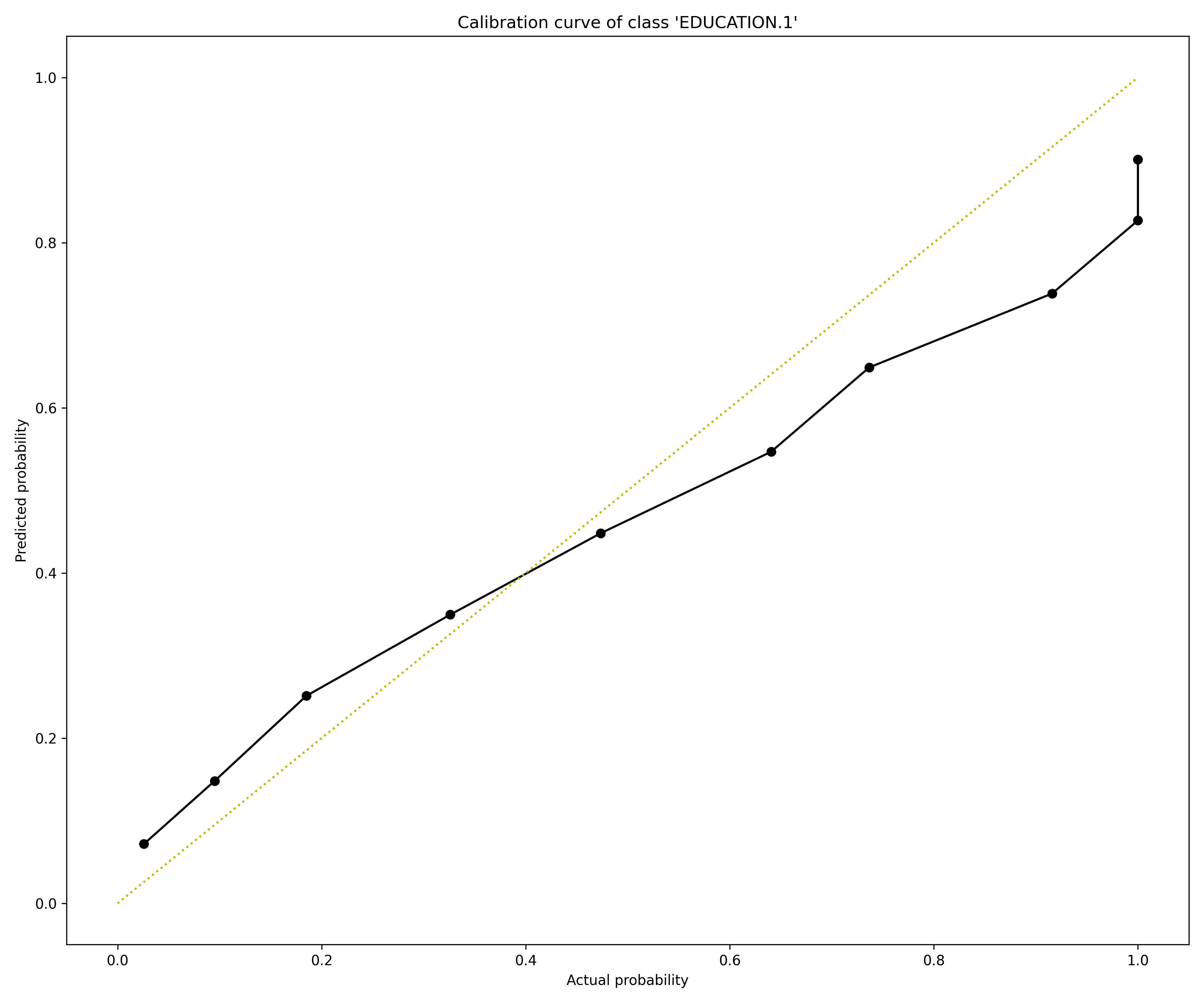
Calibration Score Explainer

This explainer is based on the calibration score H2O Model Validation test.

A calibration score test enables you to assess how well the scores generated by a classification model align with the model’s probabilities. In other words, the validation test can estimate how good the generated probabilities can be for a test dataset with real-world examples. In the case of a multi-class model, the validation test repeats the test for each target class.

Explainer utilizes the Brier score to assess the model calibration of each target class. The Brier score ranges from 0 to 1, where 0 indicates a perfect calibration. After the test, explainer assigns a Brier score to the target class (or all target classes in the case of a multi-class model).

In addition, the test generates a calibration score graph that visualizes the calibration curves to identify the ranges, directions, and magnitudes of probabilities that are off. H2O Model Validation adds a perfect calibration line (a diagonal line) for reference in this calibration score graph. Estimating how well the model is calibrated to real-world data is crucial when a classification model is used not only for complex decisions but supplies the probabilities for downstream tasks, such as pricing decisions or propensity to churn estimations.

Explainer parameters:

• worker_connection_key

  • The connection ID of the Driverless AI worker configured in the H2O Eval Studio configuration. Supported are Driverless AI servers hosted by H2O AIEM or H2O Enterprise Steam, or Driverless AI servers that use username and password authentication.

• number_of_bins

  • Defines the number of bins the explainer utilizes to divide the primary dataset.

• bin_strategy

  • Defines the binning strategy - one of uniform or quantile - the explainer utilizes to bin the primary dataset.

The explainer can be run using the Python API as follows:

# configure Driverless AI server to serve as a host of artifacts (datasets, models) and/or worker
DAI_CONNECTION = h2o_sonar_config.ConnectionConfig(
   key="local-driverless-ai-server",  # ID is generated from the connection name (NCName)
   connection_type=h2o_sonar_config.ConnectionConfigType.DRIVERLESS_AI_AIEM.name,
   name="My H2O AIEM hosted Driverless AI ",
   description="Driverless AI server hosted by H2O Enterprise AIEM.",
   server_url="https://enginemanager.cloud.h2o.ai/",
   server_id="new-dai-engine-42",
   environment_url="https://cloud.h2o.ai",
   username="firstname.lastname@h2o.ai",
   token=os.getenv(KEY_AIEM_REFRESH_TOKEN_CLOUD),
   token_use_type=h2o_sonar_config.TokenUseType.REFRESH_TOKEN.name,
)
# add the connection to the H2O Eval Studio configuration
h2o_sonar_config.config.add_connection(DAI_CONNECTION)

# run the explainer (model and datasets provided as handles as they are hosted by the Driverless AI server)
interpretation = interpret.run_interpretation(
   model=f"resource:connection:{DAI_CONNECTION.key}:key:7965e2ea-f898-11ed-b979-106530ed5ceb",
   dataset=f"resource:connection:{DAI_CONNECTION.key}:key:8965e2ea-f898-11ed-b979-106530ed5ceb",
   target_col="Weekly_Sales",
   explainers=[
      commons.ExplainerToRun(
            explainer_id=CalibrationScoreExplainer.explainer_id(),
            params={
               "worker_connection_key": DAI_CONNECTION.key,
            },
      )
   ],
   results_location="./h2o-sonar-results",
)

The explainer can be run using the command line interface (CLI) as follows:

h2o-sonar run interpretation
--explainers h2o_sonar.explainers.calibration_score_explainer.CalibrationScoreExplainer
--explainers-pars '{
   "h2o_sonar.explainers.calibration_score_explainer.CalibrationScoreExplainer": {
      "worker_connection_key": "local-driverless-ai-server",
   }
}'
--model "resource:connection:local-driverless-ai-server:key:7965e2ea-f898-11ed-b979-106530ed5ceb"
--dataset "resource:connection:local-driverless-ai-server:key:695f5d5e-f898-11ed-b979-106530ed5ceb"
--target-col "Weekly_Sales"
--results-location "./h2o-sonar-results"
--config-path "./h2o-sonar-config.json"
--encryption-key "secret-key-to-decrypt-encrypted-config-fields"

Explainer result directory description:

explainer_h2o_sonar_explainers_calibration_score_explainer_CalibrationScoreExplainer_b02fc087-110d-4b80-b1ca-3bb801bb7b2d
├── global_frame
│   ├── application_vnd_h2oai_datatable_jay
│   │   └── explanation.jay
│   └── application_vnd_h2oai_datatable_jay.meta
├── global_html_fragment
│   ├── text_html
│   │   ├── calibration_curve_0.png
│   │   ├── calibration_curve_1.png
│   │   ├── calibration_curve_2.png
│   │   ├── calibration_curve_3.png
│   │   ├── calibration_curve_4.png
│   │   ├── calibration_curve_5.png
│   │   ├── calibration_curve_6.png
│   │   └── explanation.html
│   └── text_html.meta
├── global_work_dir_archive
│   ├── application_zip
│   │   └── explanation.zip
│   └── application_zip.meta
├── log
│   └── explainer_run_b02fc087-110d-4b80-b1ca-3bb801bb7b2d.log
├── model_problems
│   └── problems_and_actions.json
├── result_descriptor.json
└── work
   ├── brier_scores.csv
   ├── calibration_curve_0.png
   ├── calibration_curve_1.png
   ├── calibration_curve_2.png
   ├── calibration_curve_3.png
   ├── calibration_curve_4.png
   ├── calibration_curve_5.png
   ├── calibration_curve_6.png
   ├── calibration_curves.csv
   ├── explanation.html
   └── mv_result.json

Explanations created by the explainer:

• global_frame

  • Calibration curve data for all classes in the datatable format.

• global_html_fragment

  • Calibration score in the HTML format.

• global_work_dir_archive

  • All explanations created by the explainer stored in a ZIP archive.

See also:

• H2O Model Validation documentation of the Calibration Score explainer

• H2O Eval Studio Model Validation Explainers

• Interpretation Directory Structure

• Library Configuration

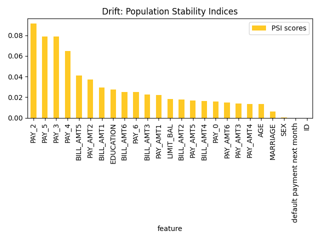
Drift Detection Explainer

This explainer is based on the drift detection H2O Model Validation test.

Drift detection refers to a validation test that enables you to identify changes in the distribution of variables in your model’s input data, preventing model performance degradation.

The explainer performs drift detection using the train and another dataset captured at different times to assess how data has changed over time. The Population Stability Index (PSI) formula is applied to each variable to measure how much the variable has shifted in distribution over time. PSI is applied to numerical and categorical columns and not date columns.

Explainer parameters:

• worker_connection_key

  • Optional connection ID of the Driverless AI worker configured in the H2O Eval Studio configuration. Supported are Driverless AI servers hosted by H2O AIEM or H2O Enterprise Steam, or Driverless AI servers that use username and password authentication.

• drift_threshold

  • Drift threshold - Problem is reported by the explainer if the drift is bigger than the threshold.

• drop_cols

  • Defines the columns to drop during the validation test. Typically drop columns refer to columns that can indicate a drift without an impact on the model, like columns not used by the model, record IDs, time columns, etc.

The explainer can be run using the Python API as follows:

# run the explainer (model and datasets provided as handles as they are hosted by the Driverless AI server)
interpretation = interpret.run_interpretation(
   # dataset might be either local or hosted by the Driverless AI server (model is not required)
   dataset="./dataset-train.csv",
   testset="./dataset-test.csv",
   model=None,
   target_col="PROFIT",
   explainers=[DriftDetection.explainer_id()],
   results_location="./h2o-sonar-results",
)

The explainer, which explains Driverless AI datasets hosted by H2O AIEM, can be run using the command line interface (CLI) as follows:

# When H2O Eval Studio loads or saves the library configuration it uses the encryption key
# to protect sensitive data - like passwords or tokens. Therefore it is convenient
# to export the encryption key as an environment variable so that it can be used
# by the library.

export H2O_SONAR_ENCRYPTION_KEY="m1-s3cr3t-k3y"

# h2o-sonar-config.json H2O Eval Studio configuration with H2O AIEM hosted Driverless AI
# connection. Note that the "token" is encrypted using the encryption key.

{
   "connections": [
      {
            "key": "my-aiem-hosted-dai-connection",
            "connection_type": "DRIVERLESS_AI_AIEM",
            "name": "My H2O AIEM hosted Driverless AI ",
            "description": "Driverless AI server hosted by H2O Enterprise AIEM.",
            "auth_server_url": "",
            "environment_url": "https://cloud.h2o.ai",
            "server_url": "https://enginemanager.cloud.h2o.ai/",
            "server_id": "new-dai-engine-42",
            "realm_name": "",
            "client_id": "",
            "token": {
               "encrypted": "gAAAAABlG-UU-...Z2iriJztlEG0l2g2rPo8RIoYiNOJMQ_CLZVp"
            },
            "token_use_type": "REFRESH_TOKEN",
            "username": "firstname.lastname@h2o.ai",
            "password": {
               "encrypted": ""
            }
      }
   ],
}

# h2o-sonar-args-run-interpretation.json file with CLI parameters stored as JSon file.
# Instead of specifying many parameters on the command line interface, it is convenient
# to store all the parameters as (reusable) JSon file.

{
   "dataset": "resource:connection:my-aiem-hosted-dai-connection:key:fb2029e6-595d-11ee-896f-6e441ddba243",
   "testset": "resource:connection:my-aiem-hosted-dai-connection:key:gb2029e6-595d-11ee-896f-6e441ddba243",
   "model": null,
   "target_col": "Weekly_Sales",
   "explainers": [
      {
            "id": "h2o_sonar.explainers.drift_explainer.DriftDetectionExplainer",
            "params": {
               "drift_threshold": 0.05,
               "worker_connection_key": "my-aiem-hosted-dai-connection"
            }
      }
   ],
   "results_location": "./results"
}

# Interperation can be run using the h2o-sonar CLI as follows:

h2o-sonar run interpretation \
   --args-as-json-location h2o-sonar-args-run-interpretation.json \
   --config-path h2o-sonar-config.json

Explainer result directory description:

explainer_h2o_sonar_explainers_drift_explainer_DriftDetectionExplainer_fee36f5d-64fb-46b3-a46a-7bbcb6007476
├── global_feature_importance
│   ├── application_json
│   │   ├── explanation.json
│   │   └── feature_importance_class_0.json
│   ├── application_json.meta
│   ├── application_vnd_h2oai_json_datatable_jay
│   │   ├── explanation.json
│   │   └── feature_importance_class_0.jay
│   └── application_vnd_h2oai_json_datatable_jay.meta
├── global_html_fragment
│   ├── text_html
│   │   ├── explanation.html
│   │   └── fi-class-0.png
│   └── text_html.meta
├── global_work_dir_archive
│   ├── application_zip
│   │   └── explanation.zip
│   └── application_zip.meta
├── log
│   └── explainer_run_fee36f5d-64fb-46b3-a46a-7bbcb6007476.log
├── model_problems
│   └── problems_and_actions.json
├── result_descriptor.json
└── work

Explanations created by the explainer:

• global_feature_importance

  • Population stability indices in JSon and datatable format.

• global_html_fragment

  • Population stability indices in the HTML format.

• global_work_dir_archive

  • All explanations created by the explainer stored in a ZIP archive.

See also:

• H2O Model Validation documentation of the Drift Detection explainer

• H2O Eval Studio Model Validation Explainers

• Interpretation Directory Structure

• Library Configuration

Segment Performance Explainer

This explainer is based on the segment performance H2O Model Validation test.

A segment performance test lets you explore a model’s data subsets (segments) that diverge from average scores. In other words, a segment performance test allows you to discover which data points (segments) the model struggles, outperformance, and performs with when generating accurate predictions.

To run a segment performance test on a model, explainer utilizes a provided dataset to generate model predictions to assess their accuracy. Explainer splits the dataset into segments by the bins of values of every variable and every pair of variables to generate results around the ability of the model to produce accurate predictions with different data segments. These results are embedded into a bubble graph that explainer generates that enables you to observe and explore data segments the model struggles, outperformance, and performs with when generating accurate predictions. For each segment, explainer calculates its size of it relative to the size of the dataset and estimates the error the model makes on the corresponding segment.

Exploring and identifying data segments in a model that do not perform as expected can lead to decisions on how you preprocess your data.

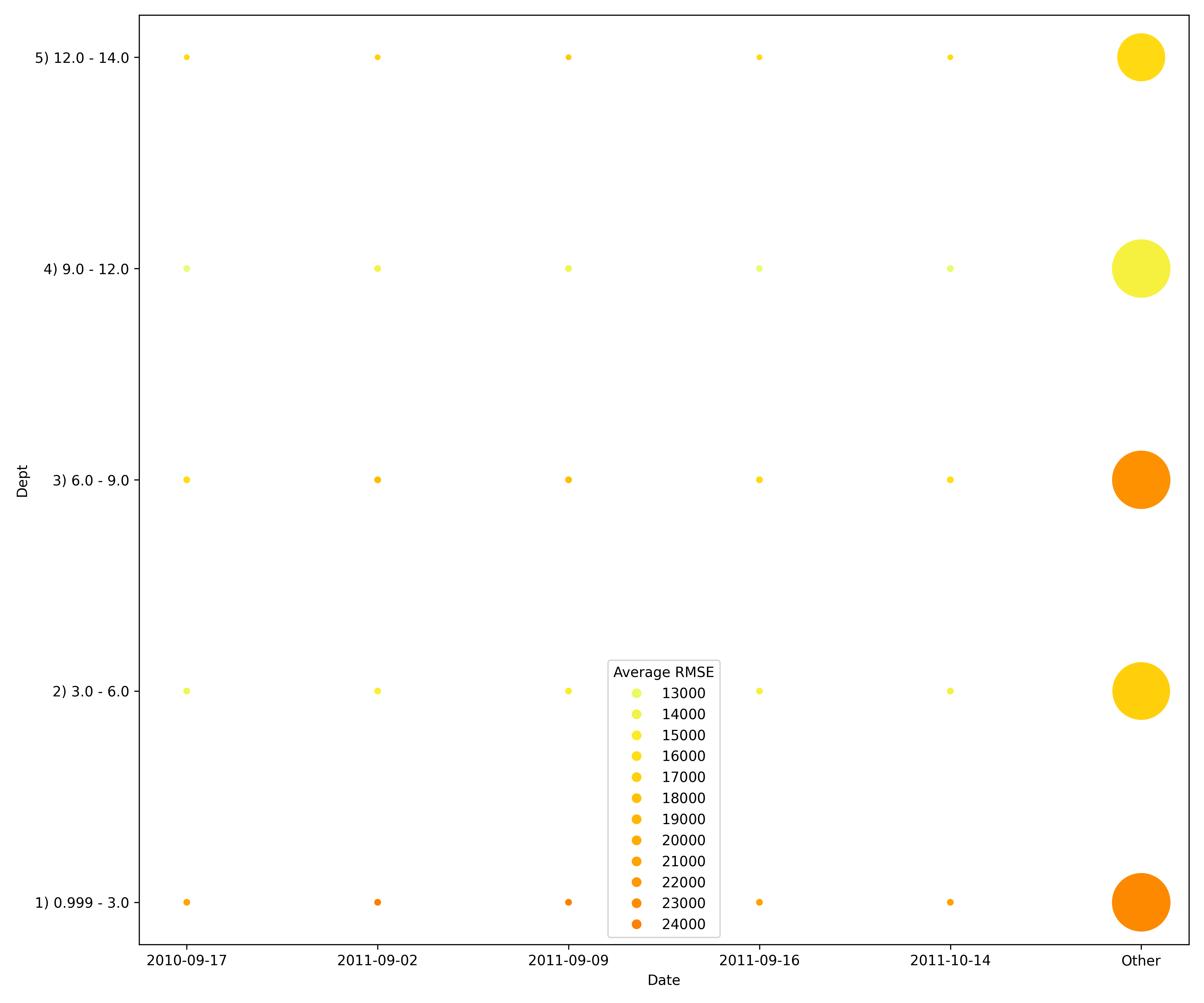
Explainer parameters:

• worker_connection_key

  • The connection ID of the Driverless AI worker configured in the H2O Eval Studio configuration. Supported are Driverless AI servers hosted by H2O AIEM or H2O Enterprise Steam, or Driverless AI servers that use username and password authentication.

• number_of_bins

  • Defines the number of bins the explainer utilizes to split the variable values of the primary dataset. In the case of a categorical column, the explainer utilizes the appropriate categories while ranging numerical columns into a specified number of bins. To run a segment performance test on a model, the explainer utilizes a provided dataset to generate model predictions to assess their accuracy. Explainer splits the dataset into segments by the bins of values of every variable and every pair of variables to generate results around the ability of the model to produce accurate predictions with different data segments. These results are embedded into a bubble graph that the explainer generates that enables you to observe and explore data segments the model struggles, outperformance, and performs with when generating accurate predictions. For each segment, explainer calculates its size of it relative to the size of the dataset and estimates the error the model makes on the corresponding segment.

• precision

  • Precision.

• drop_cols

  • Defines the columns to drop during the validation test.

The explainer can be run using the Python API as follows:

# configure Driverless AI server to serve as a host of artifacts (datasets, models) and/or worker
DAI_CONNECTION = h2o_sonar_config.ConnectionConfig(
   key="local-driverless-ai-server",  # ID is generated from the connection name (NCName)
   connection_type=h2o_sonar_config.ConnectionConfigType.DRIVERLESS_AI_AIEM.name,
   name="My H2O AIEM hosted Driverless AI ",
   description="Driverless AI server hosted by H2O Enterprise AIEM.",
   server_url="https://enginemanager.cloud.h2o.ai/",
   server_id="new-dai-engine-42",
   environment_url="https://cloud.h2o.ai",
   username="firstname.lastname@h2o.ai",
   token=os.getenv(KEY_AIEM_REFRESH_TOKEN_CLOUD),
   token_use_type=h2o_sonar_config.TokenUseType.REFRESH_TOKEN.name,
)
# add the connection to the H2O Eval Studio configuration
h2o_sonar_config.config.add_connection(DAI_CONNECTION)

# run the explainer (model and datasets provided as handles as they are hosted by the Driverless AI server)
interpretation = interpret.run_interpretation(
   model=f"resource:connection:{DAI_CONNECTION.key}:key:7965e2ea-f898-11ed-b979-106530ed5ceb",
   dataset=f"resource:connection:{DAI_CONNECTION.key}:key:8965e2ea-f898-11ed-b979-106530ed5ceb",
   testset=f"resource:connection:{DAI_CONNECTION.key}:key:9965e2ea-f898-11ed-b979-106530ed5ceb",
   target_col="Weekly_Sales",
   explainers=[
      commons.ExplainerToRun(
            explainer_id=SegmentPerformanceExplainer.explainer_id(),
            params={
               "worker_connection_key": DAI_CONNECTION.key,
               "number_of_bins": 10,
            },
      )
   ],
   results_location="./h2o-sonar-results",
)

The explainer can be run using the command line interface (CLI) as follows:

h2o-sonar run interpretation
--explainers h2o_sonar.explainers.segment_performance_explainer.SegmentPerformanceExplainer
--explainers-pars '{
   "h2o_sonar.explainers.segment_performance_explainer.SegmentPerformanceExplainer": {
      "worker_connection_key": "local-driverless-ai-server",
      "number_of_bins": 10,
   }
}'
--model "resource:connection:local-driverless-ai-server:key:7965e2ea-f898-11ed-b979-106530ed5ceb"
--dataset "resource:connection:local-driverless-ai-server:key:695f5d5e-f898-11ed-b979-106530ed5ceb"
--testset "resource:connection:local-driverless-ai-server:key:695df75c-f898-11ed-b979-106530ed5ceb"
--target-col "Weekly_Sales"
--results-location "./h2o-sonar-results"
--config-path "./h2o-sonar-config.json"
--encryption-key "secret-key-to-decrypt-encrypted-config-fields"

Explainer result directory description:

explainer_h2o_sonar_explainers_segment_performance_explainer_SegmentPerformanceExplainer_1e0e0ee1-7a1d-44da-952f-9ac574c39545
├── global_html_fragment
│   ├── text_html
│   │   ├── explanation.html
│   │   ├── scatter-0.png
│   │   ├── scatter-10.png
│   │   ├── scatter-11.png
│   │   ├── scatter-12.png
│   │   ├── scatter-13.png
│   │   ├── scatter-14.png
│   │   ├── scatter-15.png
│   │   ├── scatter-16.png
│   │   ├── scatter-17.png
│   │   ├── scatter-1.png
│   │   ├── scatter-20.png
│   │   ├── scatter-21.png
│   │   ├── scatter-22.png
│   │   ├── scatter-23.png
│   │   ├── scatter-24.png
│   │   ├── scatter-25.png
│   │   ├── scatter-26.png
│   │   ├── scatter-2.png
│   │   ├── scatter-30.png
│   │   ├── scatter-31.png
│   │   ├── scatter-32.png
│   │   ├── scatter-33.png
│   │   ├── scatter-34.png
│   │   ├── scatter-35.png
│   │   ├── scatter-3.png
│   │   ├── scatter-40.png
│   │   ├── scatter-41.png
│   │   ├── scatter-42.png
│   │   ├── scatter-43.png
│   │   ├── scatter-44.png
│   │   ├── scatter-4.png
│   │   ├── scatter-50.png
│   │   ├── scatter-51.png
│   │   ├── scatter-52.png
│   │   ├── scatter-53.png
│   │   ├── scatter-5.png
│   │   ├── scatter-60.png
│   │   ├── scatter-61.png
│   │   ├── scatter-62.png
│   │   ├── scatter-6.png
│   │   ├── scatter-70.png
│   │   ├── scatter-71.png
│   │   ├── scatter-7.png
│   │   ├── scatter-80.png
│   │   └── scatter-8.png
│   └── text_html.meta
├── global_work_dir_archive
│   ├── application_zip
│   │   └── explanation.zip
│   └── application_zip.meta
├── log
│   └── explainer_run_1e0e0ee1-7a1d-44da-952f-9ac574c39545.log
├── model_problems
│   └── problems_and_actions.json
├── result_descriptor.json
└── work
   ├── explanation.html
   └── segment-performance.csv

Explanations created by the explainer:

• global_html_fragment

  • Adversarial similarity in the HTML format.

• global_work_dir_archive

  • All explanations created by the explainer stored in a ZIP archive.

See also:

• H2O Model Validation documentation of the Segment performance explainer

• H2O Eval Studio Model Validation Explainers

• Interpretation Directory Structure

• Library Configuration

Size Dependency Explainer

This explainer is based on the size dependency H2O Model Validation test.

A size dependency test enables you to analyze the effects different sizes of train data will have on the accuracy of a selected model. In particular, size dependency facilitates model stability analysis and, for example, can answer whether augmenting an existing train data seems to be promising in terms of model accuracy.

Explainer selects an appropriate sampling technique for the size dependency test based on the selected model type. Available sampling techniques are as follows:

• Random sampling

  • Explainer uses a random sampling technique to create new sub-training samples for independent and identically distributed (IID) models

• Expanding window sampling

  • Explainer uses a expanding window sampling technique to create new sub-training samples for time series models while utilizing time columns to ensure that sub-training samples grow from recent to oldest data

For either sampling technique (random or expanding window), before it is applied, the original train data is split using folds that improve generalization and data balance when one of the sampling techniques is applied while using folds.

In the case of IID models, folds and sub-training samples are created at random, but for time series models, folds and sub-training samples are created using a time column to ensure that sub-training samples grow from the most recent to oldest data points.

Based on the number of folds (N), explainer retrains the model N times by only updating its training dataset with the new sub-training samples while generating a scorer for each iteration of the retraining process for further analysis.

Sampling the original training data for a model under random or expanding window sampling can be illustrated in the below image when N (folds) equals 4.

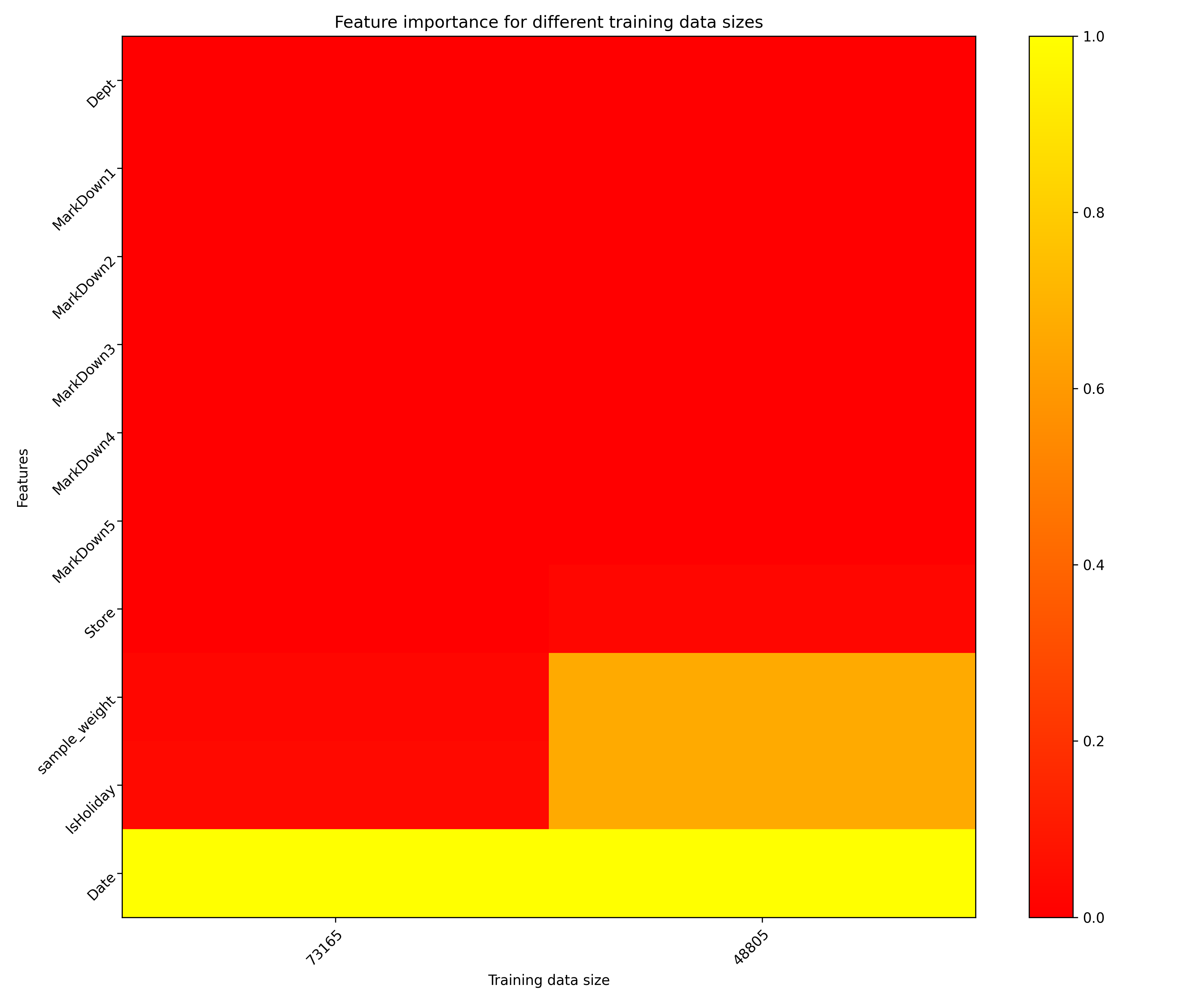
Explainer parameters:

• worker_connection_key

  • The connection ID of the Driverless AI worker configured in the H2O Eval Studio configuration. Supported are Driverless AI servers hosted by H2O AIEM or H2O Enterprise Steam, or Driverless AI servers that use username and password authentication.

• time_col

  • Defines the time column of the primary and secondary dataset, which explainer utilizes to perform time-based splits.

• number_of_splits

  • Defines the number of splits that explainer performs on the primary dataset to assess dataset size dependency.

• worker_cleanup

  • Determines if the explainer should delete the artifacts created in the worker. In this case, artifacts refer to experiments and datasets generated during the backtesting validation test. By default, explainer checks this setting (enables it), and accordingly, H2O Model Validation deletes all artifacts because they are no longer needed after the validation test is complete.

• plot_type

  • Plot type to be used for Partial Dependence rendering - heatmap, contour-3d or surface-3d.

The explainer can be run using the Python API as follows:

# configure Driverless AI server to serve as a host of artifacts (datasets, models) and/or worker
DAI_CONNECTION = h2o_sonar_config.ConnectionConfig(
   key="local-driverless-ai-server",  # ID is generated from the connection name (NCName)
   connection_type=h2o_sonar_config.ConnectionConfigType.DRIVERLESS_AI_AIEM.name,
   name="My H2O AIEM hosted Driverless AI ",
   description="Driverless AI server hosted by H2O Enterprise AIEM.",
   server_url="https://enginemanager.cloud.h2o.ai/",
   server_id="new-dai-engine-42",
   environment_url="https://cloud.h2o.ai",
   username="firstname.lastname@h2o.ai",
   token=os.getenv(KEY_AIEM_REFRESH_TOKEN_CLOUD),
   token_use_type=h2o_sonar_config.TokenUseType.REFRESH_TOKEN.name,
)
# add the connection to the H2O Eval Studio configuration
h2o_sonar_config.config.add_connection(DAI_CONNECTION)

# run the explainer (model and datasets provided as handles as they are hosted by the Driverless AI server)
interpretation = interpret.run_interpretation(
   model=f"resource:connection:{DAI_CONNECTION.key}:key:7965e2ea-f898-11ed-b979-106530ed5ceb",
   dataset=f"resource:connection:{DAI_CONNECTION.key}:key:8965e2ea-f898-11ed-b979-106530ed5ceb",
   testset=f"resource:connection:{DAI_CONNECTION.key}:key:9965e2ea-f898-11ed-b979-106530ed5ceb",
   target_col="Weekly_Sales",
   explainers=[
      commons.ExplainerToRun(
            explainer_id=SizeDependencyExplainer.explainer_id(),
            params={
               "worker_connection_key": DAI_CONNECTION.key,
               "time_col": "Date",
            },
      )
   ],
   results_location="./h2o-sonar-results",
)

The explainer can be run using the command line interface (CLI) as follows:

h2o-sonar run interpretation
--explainers h2o_sonar.explainers.size_dependency_explainer.SizeDependencyExplainer
--explainers-pars '{
   "h2o_sonar.explainers.size_dependency_explainer.SizeDependencyExplainer": {
      "worker_connection_key": "local-driverless-ai-server",
      "time_col": "Date",
   }
}'
--model "resource:connection:local-driverless-ai-server:key:7965e2ea-f898-11ed-b979-106530ed5ceb"
--dataset "resource:connection:local-driverless-ai-server:key:695f5d5e-f898-11ed-b979-106530ed5ceb"
--testset "resource:connection:local-driverless-ai-server:key:695df75c-f898-11ed-b979-106530ed5ceb"
--target-col "Weekly_Sales"
--results-location "./h2o-sonar-results"
--config-path "./h2o-sonar-config.json"
--encryption-key "secret-key-to-decrypt-encrypted-config-fields"

Explainer result directory description:

explainer_h2o_sonar_explainers_size_dependency_explainer_SizeDependencyExplainer_4d0ec4b4-38a7-4606-80a9-235e827532b7
├── global_3d_data
│   ├── application_json
│   │   ├── data3d_feature_0_class_0.json
│   │   └── explanation.json
│   ├── application_json.meta
│   ├── application_vnd_h2oai_json_csv
│   │   ├── data3d_feature_0_class_0.csv
│   │   └── explanation.json
│   └── application_vnd_h2oai_json_csv.meta
├── global_html_fragment
│   ├── text_html
│   │   ├── explanation.html
│   │   └── heatmap.png
│   └── text_html.meta
├── global_work_dir_archive
│   ├── application_zip
│   │   └── explanation.zip
│   └── application_zip.meta
├── log
│   └── explainer_run_4d0ec4b4-38a7-4606-80a9-235e827532b7.log
├── model_problems
│   └── problems_and_actions.json
├── result_descriptor.json
└── work
   ├── explanation.html
   └── heatmap.png

Explanations created by the explainer:

• global_3d_data

  • Feature importance for different training data sizes in JSon, CSV and datatable formats.

• global_html_fragment

  • Feature importance for different training data sizes in the HTML format.

• global_work_dir_archive

  • All explanations created by the explainer stored in a ZIP archive.

See also:

• H2O Model Validation documentation of the Size Dependency explainer

• H2O Eval Studio Model Validation Explainers

• Interpretation Directory Structure

• Library Configuration